Multiple Categorical Predictors
Add more than one categorical predictor
Let’s explore the ability to add more than one categorical predictor to our model. This will then build into thinking through interactions. Let’s load some new data. These are bike data from Philadelphia program, called Indego. The data loaded below are from Q3 of 2023.
Here is information about the columns in the data.
- trip_id: Locally unique integer that identifies the trip
- duration: Length of trip in minutes
- start_time: The date/time when the trip began, presented in ISO 8601 format in local time
- end_time: The date/time when the trip ended, presented in ISO 8601 format in local time
- start_station: The station ID where the trip originated (for station name and more information on each station see the Station Table)
- start_lat: The latitude of the station where the trip originated
- start_lon: The longitude of the station where the trip originated
- end_station: The station ID where the trip terminated (for station name and more information on each station see the Station Table)
- end_lat: The latitude of the station where the trip terminated
- end_lon: The longitude of the station where the trip terminated
- bike_id: Locally unique integer that identifies the bike
- plan_duration: The number of days that the plan the passholder is using entitles them to ride; 0 is used for a single ride plan (Walk-up)
- trip_route_category: “Round Trip” for trips starting and ending at the same station or “One Way” for all other trips
- passholder_type: The name of the passholder’s plan
- bike_type: The kind of bike used on the trip, including standard pedal-powered bikes or electric assist bikes
library(tidyverse)## ── Attaching core tidyverse packages ──────────────────────── tidyverse 2.0.0 ──
## ✔ dplyr 1.1.4 ✔ readr 2.1.5
## ✔ forcats 1.0.0 ✔ stringr 1.5.1
## ✔ ggplot2 3.4.4 ✔ tibble 3.2.1
## ✔ lubridate 1.9.3 ✔ tidyr 1.3.1
## ✔ purrr 1.0.2
## ── Conflicts ────────────────────────────────────────── tidyverse_conflicts() ──
## ✖ dplyr::filter() masks stats::filter()
## ✖ dplyr::lag() masks stats::lag()
## ℹ Use the conflicted package (<http://conflicted.r-lib.org/>) to force all conflicts to become errorslibrary(ggformula)## Loading required package: scales
##
## Attaching package: 'scales'
##
## The following object is masked from 'package:purrr':
##
## discard
##
## The following object is masked from 'package:readr':
##
## col_factor
##
## Loading required package: ggridges
##
## New to ggformula? Try the tutorials:
## learnr::run_tutorial("introduction", package = "ggformula")
## learnr::run_tutorial("refining", package = "ggformula")theme_set(theme_bw(base_size = 18))
temp <- tempfile()
download.file("https://bicycletransit.wpenginepowered.com/wp-content/uploads/2023/10/indego-trips-2023-q3.zip", temp)
bike <- readr::read_csv(unz(temp, "indego-trips-2023-q3-2.csv")) |>
filter(duration <= 120 & passholder_type != 'Walk-up')## Warning: One or more parsing issues, call `problems()` on your data frame for details,
## e.g.:
## dat <- vroom(...)
## problems(dat)## Rows: 353256 Columns: 15
## ── Column specification ────────────────────────────────────────────────────────
## Delimiter: ","
## chr (5): start_time, end_time, trip_route_category, passholder_type, bike_type
## dbl (10): trip_id, duration, start_station, start_lat, start_lon, end_statio...
##
## ℹ Use `spec()` to retrieve the full column specification for this data.
## ℹ Specify the column types or set `show_col_types = FALSE` to quiet this message.unlink(temp)
head(bike)## # A tibble: 6 × 15
## trip_id duration start_time end_time start_station start_lat start_lon
## <dbl> <dbl> <chr> <chr> <dbl> <dbl> <dbl>
## 1 677293140 2 7/1/2023 0:00 7/1/2023 0… 3271 39.9 -75.2
## 2 677304406 27 7/1/2023 0:00 7/1/2023 0… 3060 40.0 -75.2
## 3 677304584 32 7/1/2023 0:00 7/1/2023 0… 3057 40.0 -75.2
## 4 677302282 6 7/1/2023 0:00 7/1/2023 0… 3038 39.9 -75.2
## 5 677304444 27 7/1/2023 0:01 7/1/2023 0… 3060 40.0 -75.2
## 6 677303703 9 7/1/2023 0:01 7/1/2023 0… 3158 39.9 -75.2
## # ℹ 8 more variables: end_station <dbl>, end_lat <dbl>, end_lon <dbl>,
## # bike_id <dbl>, plan_duration <dbl>, trip_route_category <chr>,
## # passholder_type <chr>, bike_type <chr>dim(bike)## [1] 351189 15Suppose we were interested in the following research questions.
- Does the trip route, type of pass, and bike type explain variation in the duration the bike was rented?
Let’s explore this descriptively.
gf_density(~ duration, data = bike) |>
  gf_labs(x = "Duration, in minutes")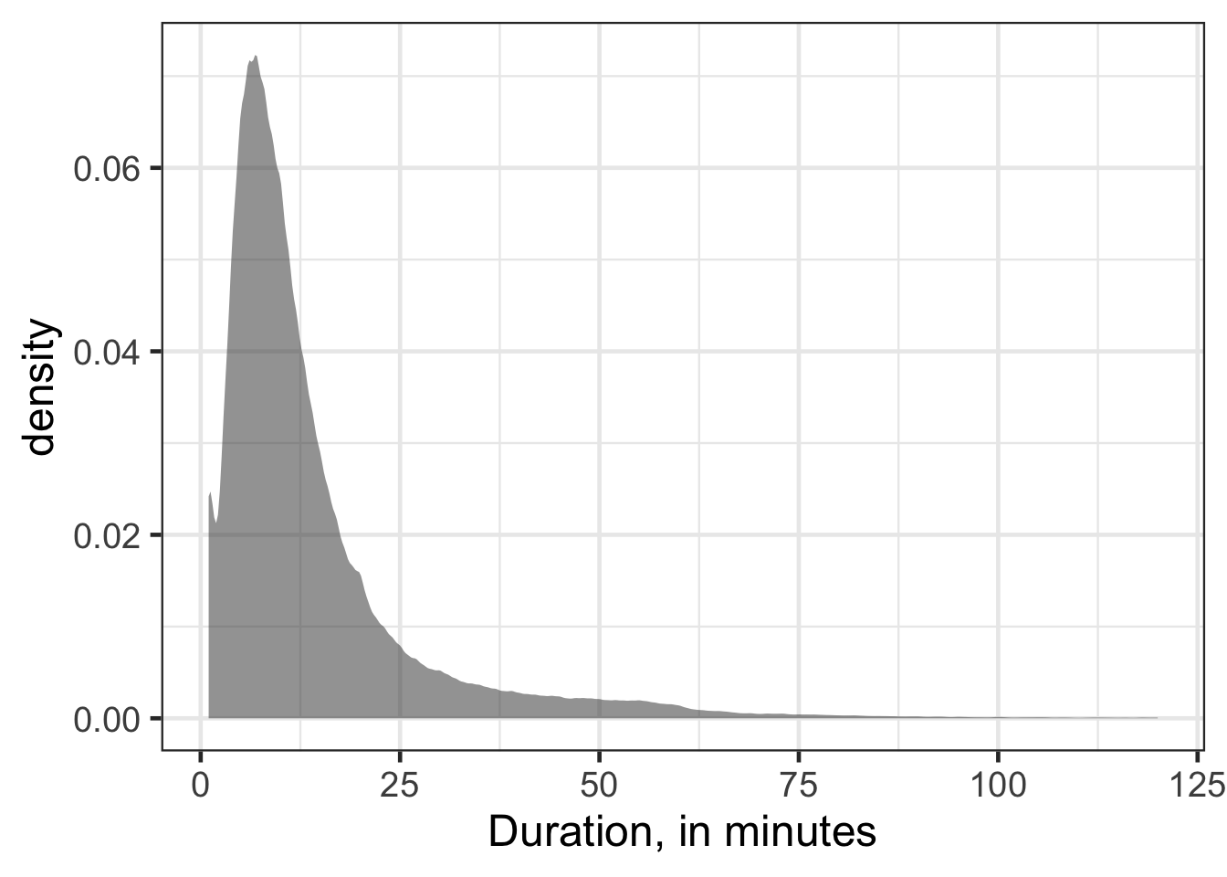
gf_violin(bike_type ~ duration, data = bike, fill = 'gray85', draw_quantiles = c(0.1, 0.5, 0.9)) |>
gf_labs(x = "Duration, in minutes", y = "") 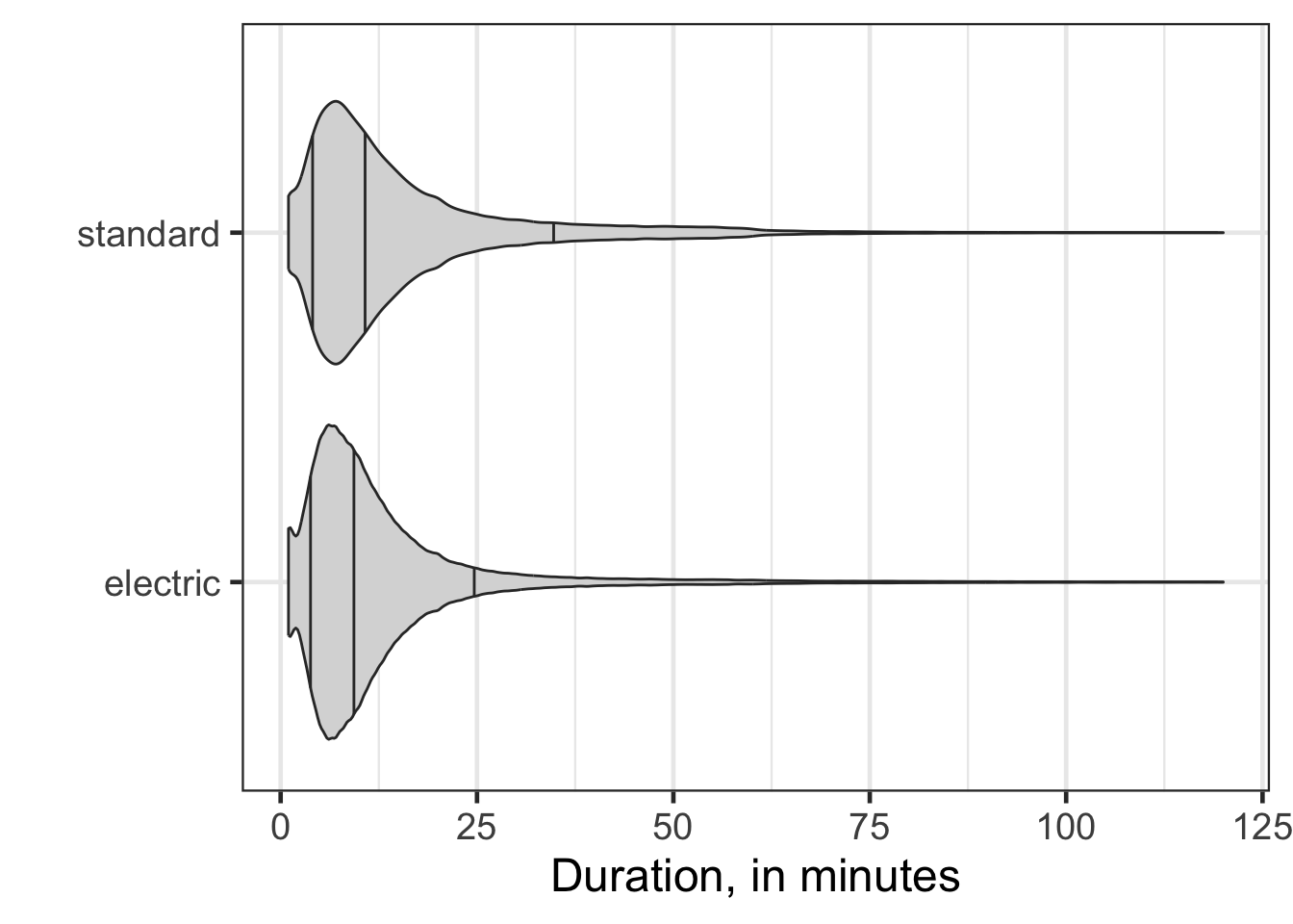
gf_violin(passholder_type ~ duration, data = bike, fill = 'gray85', draw_quantiles = c(0.1, 0.5, 0.9)) |>
gf_labs(x = "Duration, in minutes", y = "") 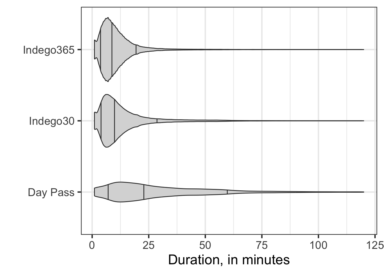
gf_violin(trip_route_category ~ duration, data = bike, fill = 'gray85', draw_quantiles = c(0.1, 0.5, 0.9)) |>
gf_labs(x = "Duration, in minutes", y = "") 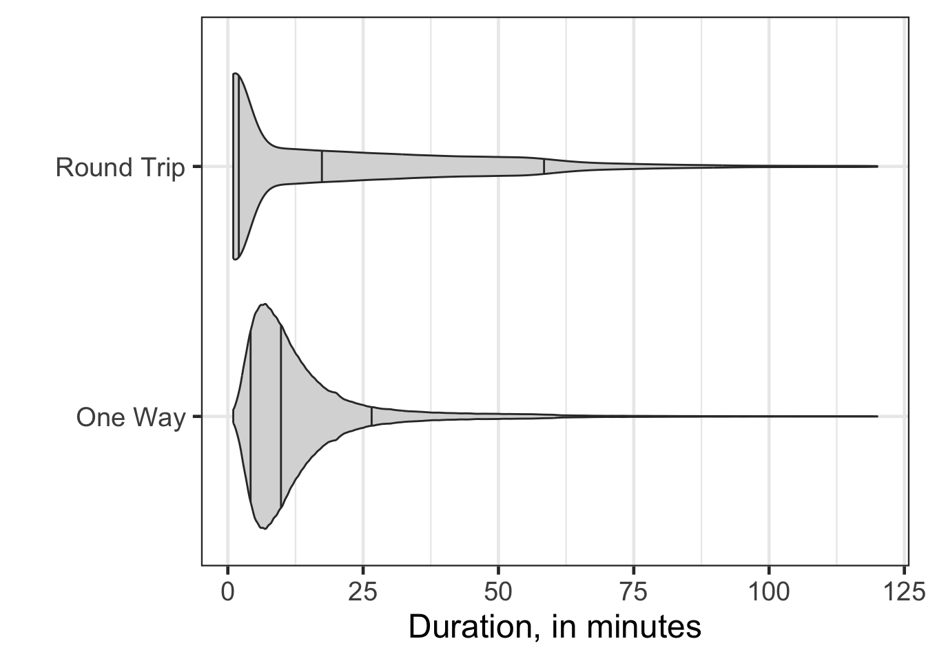
Regression model with multiple categorical predictors
Similar to multiple linear regression, including multiple categorical predictors is similar to that case. The simplest model is the additive model, also commonly referred to as the main effect model. Let’s start with two categorical attributes that take on two different values.
\[ duration = \beta_{0} + \beta_{1} bike\_type + \beta_{2} trip\_route\_category + \epsilon \]
bike_lm <- lm(duration ~ bike_type + trip_route_category, data = bike)

broom::glance(bike_lm)
## # A tibble: 1 × 12
## r.squared adj.r.squared sigma statistic p.value df logLik AIC BIC
## <dbl> <dbl> <dbl> <dbl> <dbl> <dbl> <dbl> <dbl> <dbl>
## 1 0.0214 0.0214 13.6 3832. 0 2 -1414715. 2.83e6 2.83e6
## # ℹ 3 more variables: deviance <dbl>, df.residual <int>, nobs <int>broom::tidy(bike_lm) |>
mutate_if(is.double, round, 3)## # A tibble: 3 × 5
## term estimate std.error statistic p.value
## <chr> <dbl> <dbl> <dbl> <dbl>
## 1 (Intercept) 12.5 0.032 393. 0
## 2 bike_typestandard 2.49 0.046 54.1 0
## 3 trip_route_categoryRound Trip 6.00 0.088 68.4 0two_way_predict <- broom::augment(bike_lm) |>
distinct(bike_type, trip_route_category, .fitted)
two_way_predict## # A tibble: 4 × 3
## bike_type trip_route_category .fitted
## <chr> <chr> <dbl>
## 1 electric One Way 12.5
## 2 standard One Way 15.0
## 3 electric Round Trip 18.5
## 4 standard Round Trip 21.0mean_duration <- df_stats(duration ~ bike_type + trip_route_category, data =bike, mean, length)
mean_duration## response bike_type trip_route_category mean length
## 1 duration electric One Way 12.62121 176083
## 2 duration standard One Way 14.88991 149160
## 3 duration electric Round Trip 17.21428 13674
## 4 duration standard Round Trip 22.46178 12272gf_point(.fitted ~ bike_type, color = ~ trip_route_category, data = two_way_predict, size = 5) |>
gf_line(size = 1.5, group = ~ trip_route_category) |>
gf_labs(x = "", y = "Model Predicted Values", color = 'Trip Route') |>
gf_point(mean ~ bike_type, color = ~ trip_route_category, data = mean_duration, shape = 15, size = 5)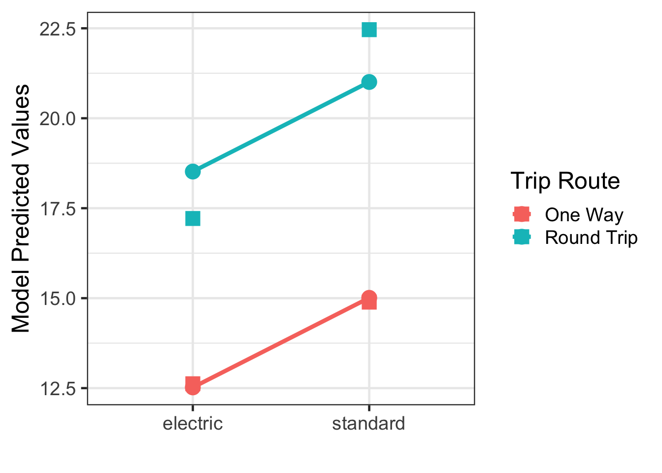
Back to the coefficients to really understand what these are.
broom::tidy(bike_lm) |>
  mutate_if(is.double, round, 3)
## # A tibble: 3 × 5
## term estimate std.error statistic p.value
## <chr> <dbl> <dbl> <dbl> <dbl>
## 1 (Intercept) 12.5 0.032 393. 0
## 2 bike_typestandard 2.49 0.046 54.1 0
## 3 trip_route_categoryRound Trip 6.00 0.088 68.4 0- Intercept: The average bike rental duration for the reference group (electric bikes and one-way trips).
- bike_typestandard: This is like a slope, so for a one unit change in bike type (ie, moving from an electric bike to a standard bike), the estimated mean change in bike duration decreased by 0.375 minutes, holding other attributes constant.
- trip_route_categoryRound Trip: This is again like a slope, for a one unit change in trip route (ie, moving from a one-way trip to a round trip), the estimated mean change in bike duraction increased by 7.246 minutes, holder other attributes constant.
These are like weighted marginal means, where the weighting is occuring due to different sample sizes among the groups.
count(bike, bike_type, trip_route_category)## # A tibble: 4 × 3
## bike_type trip_route_category n
## <chr> <chr> <int>
## 1 electric One Way 176083
## 2 electric Round Trip 13674
## 3 standard One Way 149160
## 4 standard Round Trip 12272df_stats(duration ~ bike_type + trip_route_category, data = bike, mean) |>
pivot_wider(names_from = 'trip_route_category', values_from = "mean")## # A tibble: 2 × 4
## response bike_type `One Way` `Round Trip`
## <chr> <chr> <dbl> <dbl>
## 1 duration electric 12.6 17.2
## 2 duration standard 14.9 22.5Interaction Model
The interaction model expands on the main effect only model, by allowing the effect of one category to differ based on elements of the other category. One way to think about this in the case with two categorical attributes, is that the mean change differs based on levels of the second attribute. This model, in the case where the attributes are each two groups, adds one additional term.
\[ duration = \beta_{0} + \beta_{1} bike\_type + \beta_{2} trip\_route\_category + \beta_{3} bike\_type:trip\_route\_category + \epsilon \]
bike_lm_int <- lm(duration ~ bike_type + trip_route_category + bike_type:trip_route_category, data = bike)

broom::glance(bike_lm_int)
## # A tibble: 1 × 12
## r.squared adj.r.squared sigma statistic p.value df logLik AIC BIC
## <dbl> <dbl> <dbl> <dbl> <dbl> <dbl> <dbl> <dbl> <dbl>
## 1 0.0222 0.0221 13.6 2653. 0 3 -1414571. 2.83e6 2.83e6
## # ℹ 3 more variables: deviance <dbl>, df.residual <int>, nobs <int>broom::tidy(bike_lm_int) |>
mutate_if(is.double, round, 3)## # A tibble: 4 × 5
## term estimate std.error statistic p.value
## <chr> <dbl> <dbl> <dbl> <dbl>
## 1 (Intercept) 12.6 0.032 390. 0
## 2 bike_typestandard 2.27 0.048 47.5 0
## 3 trip_route_categoryRound Trip 4.59 0.121 38.1 0
## 4 bike_typestandard:trip_route_categoryRou… 2.98 0.176 17.0 0two_way_predict_int <- broom::augment(bike_lm_int) |>
distinct(bike_type, trip_route_category, .fitted)
two_way_predict_int## # A tibble: 4 × 3
## bike_type trip_route_category .fitted
## <chr> <chr> <dbl>
## 1 electric One Way 12.6
## 2 standard One Way 14.9
## 3 electric Round Trip 17.2
## 4 standard Round Trip 22.5gf_point(.fitted ~ bike_type, color = ~ trip_route_category, data = two_way_predict_int, size = 5) |>
gf_line(size = 1.5, group = ~ trip_route_category) |>
gf_labs(x = "", y = "Model Predicted Values", color = 'Trip Route') |>
gf_point(mean ~ bike_type, color = ~ trip_route_category, data = mean_duration, shape = 15, size = 5)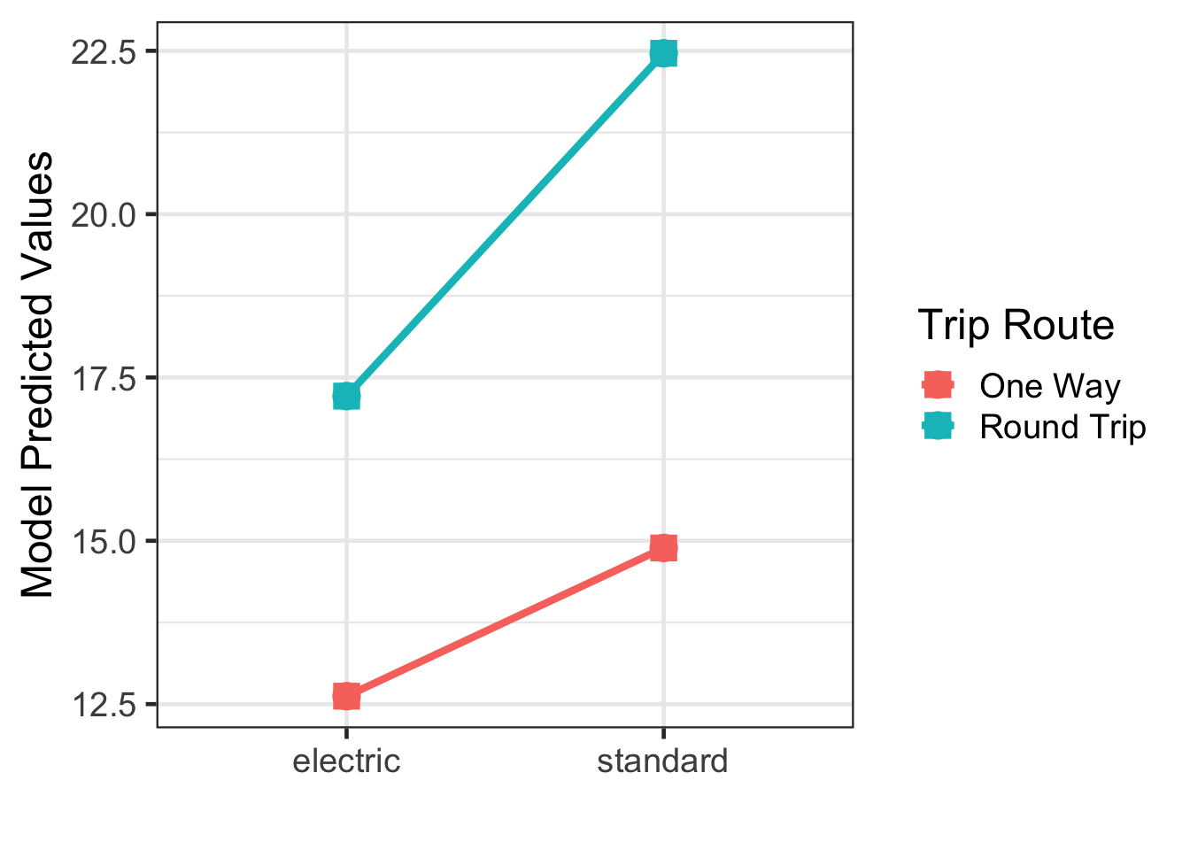
Back to the coefficients and what do these mean here.
broom::tidy(bike_lm_int)  |>
  mutate_if(is.double, round, 3)
## # A tibble: 4 × 5
## term estimate std.error statistic p.value
## <chr> <dbl> <dbl> <dbl> <dbl>
## 1 (Intercept) 12.6 0.032 390. 0
## 2 bike_typestandard 2.27 0.048 47.5 0
## 3 trip_route_categoryRound Trip 4.59 0.121 38.1 0
## 4 bike_typestandard:trip_route_categoryRou… 2.98 0.176 17.0 0- Intercept: The average bike rental duration for the reference group (electric bikes and one-way trips).
- bike_typestandard: This is like a slope, so for a one unit change in bike type (ie, moving from an electric bike to a standard bike), the estimated mean change in bike duration decreased by .05 minutes, holding other attributes constant.
- trip_route_categoryRound Trip: This is again like a slope, for a one unit change in trip route (ie, moving from a one-way trip to a round trip), the estimated mean change in bike duraction increased by 4.3 minutes, holder other attributes constant.
- bike_typestandard:trip_route_categoryRound Trip: This is the interaction effect and is the additional mean level change for standard bikes and round trips, holding other attributes constant.
We can get the estimated means for the 4 groups as follows:
\[ \hat{\mu}_{elec-1way} = 15.2 \] \[ \hat{\mu}_{elec-RT} = 15.2 + 4.3 \] \[ \hat{\mu}_{stand-1way} = 15.2 - .05 \] \[ \hat{\mu}_{stand-RT} = 15.2 - 0.05 + 4.3 + 4.7 \]
Example
What about the example with two categorical attributes bike type and passholder type? Fit this model below and interpret the parameter estimates, both one without and with interaction effects.
Second order (three-way) interaction
The more attributes that interact with one another makes the model more complicated and difficult to interpret. Still, let’s try a second order or three way interaction.
bike_lm_3way <- lm(duration ~ bike_type * trip_route_category * passholder_type, data = bike)

broom::glance(bike_lm_3way)
## # A tibble: 1 × 12
## r.squared adj.r.squared sigma statistic p.value df logLik AIC BIC
## <dbl> <dbl> <dbl> <dbl> <dbl> <dbl> <dbl> <dbl> <dbl>
## 1 0.112 0.112 12.9 4035. 0 11 -1397605. 2.80e6 2.80e6
## # ℹ 3 more variables: deviance <dbl>, df.residual <int>, nobs <int>broom::tidy(bike_lm_3way) |>
mutate_if(is.double, round, 3)## # A tibble: 12 × 5
## term estimate std.error statistic p.value
## <chr> <dbl> <dbl> <dbl> <dbl>
## 1 (Intercept) 27.4 0.12 229. 0
## 2 bike_typestandard 0.256 0.189 1.35 0.177
## 3 trip_route_categoryRound Trip 6.74 0.284 23.7 0
## 4 passholder_typeIndego30 -15.5 0.126 -123. 0
## 5 passholder_typeIndego365 -17.1 0.136 -125. 0
## 6 bike_typestandard:trip_route_categoryRo… -0.851 0.46 -1.85 0.064
## 7 bike_typestandard:passholder_typeIndego… 3.28 0.197 16.6 0
## 8 bike_typestandard:passholder_typeIndego… 0.718 0.209 3.44 0.001
## 9 trip_route_categoryRound Trip:passholde… -4.34 0.317 -13.7 0
## 10 trip_route_categoryRound Trip:passholde… -8.16 0.41 -19.9 0
## 11 bike_typestandard:trip_route_categoryRo… 5.49 0.502 10.9 0
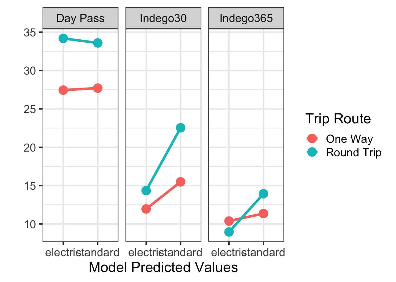
## 12 bike_typestandard:trip_route_categoryRo… 4.85 0.619 7.84 0Interpreting these coefficients can be challenging, visualizing them can be a more effective way to undersand the impact these may have. The following steps will be used to visualize these model results:
- Generate model-implied or predicted values for each combination of model values
- Plot those model implied means
three_way_predict_int <- broom::augment(bike_lm_3way) |>
   distinct(bike_type, trip_route_category, passholder_type, .fitted)

three_way_predict_int
## # A tibble: 12 × 4
## bike_type trip_route_category passholder_type .fitted
## <chr> <chr> <chr> <dbl>
## 1 electric One Way Indego30 12.0
## 2 standard One Way Indego30 15.5
## 3 standard One Way Day Pass 27.7
## 4 electric One Way Indego365 10.4
## 5 standard One Way Indego365 11.4
## 6 electric One Way Day Pass 27.4
## 7 electric Round Trip Indego30 14.4
## 8 standard Round Trip Day Pass 33.6
## 9 standard Round Trip Indego365 13.9
## 10 standard Round Trip Indego30 22.5
## 11 electric Round Trip Day Pass 34.2
## 12 electric Round Trip Indego365 8.96gf_point(.fitted ~ bike_type, color = ~ trip_route_category, data = three_way_predict_int, size = 5) |>
gf_line(size = 1.5, group = ~ trip_route_category) |>
gf_facet_wrap(~ passholder_type) |>
gf_labs(y = "", x = "Model Predicted Values", color = 'Trip Route')