Pairwise Contrasts
More details on pairwise contrasts
Last week the idea of pairwise contrasts were introduced. Here is a more formal discussion of pairwise contrasts and controlling of familywise type I error rates.
Bonferroni Method
This method is introduced first, primarily due to its simplicity. This is not the best measure to use however as will be discussed below. The Bonferroni method makes the following adjustment:
\[ \alpha_{new} = \frac{\alpha}{m} \]
Where \(m\) is the number of hypotheses being tested. Let’s use a specific example to frame this based on the baseball data.
library(tidyverse)## ── Attaching core tidyverse packages ──────────────────────── tidyverse 2.0.0 ──
## ✔ dplyr 1.1.4 ✔ readr 2.1.5
## ✔ forcats 1.0.0 ✔ stringr 1.5.1
## ✔ ggplot2 3.4.4 ✔ tibble 3.2.1
## ✔ lubridate 1.9.3 ✔ tidyr 1.3.1
## ✔ purrr 1.0.2
## ── Conflicts ────────────────────────────────────────── tidyverse_conflicts() ──
## ✖ dplyr::filter() masks stats::filter()
## ✖ dplyr::lag() masks stats::lag()
## ℹ Use the conflicted package (<http://conflicted.r-lib.org/>) to force all conflicts to become errorslibrary(Lahman)
library(ggformula)## Loading required package: scales
##
## Attaching package: 'scales'
##
## The following object is masked from 'package:purrr':
##
## discard
##
## The following object is masked from 'package:readr':
##
## col_factor
##
## Loading required package: ggridges
##
## New to ggformula? Try the tutorials:
## learnr::run_tutorial("introduction", package = "ggformula")
## learnr::run_tutorial("refining", package = "ggformula")theme_set(theme_bw(base_size = 18))
career <- Batting |>
filter(AB > 100) |>
anti_join(Pitching, by = "playerID") |>
filter(yearID > 1990) |>
group_by(playerID, lgID) |>
summarise(H = sum(H), AB = sum(AB)) |>
mutate(average = H / AB)## `summarise()` has grouped output by 'playerID'. You can override using the
## `.groups` argument.career <- Appearances |>
filter(yearID > 1990) |>
select(-GS, -G_ph, -G_pr, -G_batting, -G_defense, -G_p, -G_lf, -G_cf, -G_rf) |>
rowwise() |>
mutate(g_inf = sum(c_across(G_1b:G_ss))) |>
select(-G_1b, -G_2b, -G_3b, -G_ss) |>
group_by(playerID, lgID) |>
summarise(catcher = sum(G_c),
outfield = sum(G_of),
dh = sum(G_dh),
infield = sum(g_inf),
total_games = sum(G_all)) |>
pivot_longer(catcher:infield,
names_to = "position") |>
filter(value > 0) |>
group_by(playerID, lgID) |>
slice_max(value) |>
select(playerID, lgID, position) |>
inner_join(career)## `summarise()` has grouped output by 'playerID'. You can override using the
## `.groups` argument.
## Joining with `by = join_by(playerID, lgID)`career <- People |>
tbl_df() |>
dplyr::select(playerID, nameFirst, nameLast) |>
unite(name, nameFirst, nameLast, sep = " ") |>
inner_join(career, by = "playerID")## Warning: `tbl_df()` was deprecated in dplyr 1.0.0.
## ℹ Please use `tibble::as_tibble()` instead.
## Call `lifecycle::last_lifecycle_warnings()` to see where this warning was
## generated.career <- career |>
mutate(league_dummy = ifelse(lgID == 'NL', 1, 0))
head(career)## # A tibble: 6 × 8
## playerID name lgID position H AB average league_dummy
## <chr> <chr> <fct> <chr> <int> <int> <dbl> <dbl>
## 1 abbotje01 Jeff Abbott AL outfield 127 459 0.277 0
## 2 abbotku01 Kurt Abbott AL infield 33 123 0.268 0
## 3 abbotku01 Kurt Abbott NL infield 455 1780 0.256 1
## 4 abercre01 Reggie Abercrombie NL outfield 54 255 0.212 1
## 5 abernbr01 Brent Abernathy AL infield 194 767 0.253 0
## 6 abnersh01 Shawn Abner AL outfield 81 309 0.262 0position_lm <- lm(average ~ 1 + position, data = career)
broom::tidy(position_lm)## # A tibble: 4 × 5
## term estimate std.error statistic p.value
## <chr> <dbl> <dbl> <dbl> <dbl>
## 1 (Intercept) 0.241 0.00140 172. 0
## 2 positiondh 0.0144 0.00344 4.19 2.88e- 5
## 3 positioninfield 0.0122 0.00162 7.57 5.03e-14
## 4 positionoutfield 0.0138 0.00164 8.44 4.97e-17count(career, position)## # A tibble: 4 × 2
## position n
## <chr> <int>
## 1 catcher 415
## 2 dh 83
## 3 infield 1279
## 4 outfield 1165Given that there are 4 groups, if all pairwise comparisons were of interest, the following would be all possible NULL hypotheses. Note, I am assuming that each of these has a matching alternative hypothesis that states the groups differences are different from 0.
\[ H_{0}: \mu_{catcher} - \mu_{dh} = 0 \\ H_{0}: \mu_{catcher} - \mu_{infield} = 0 \\ H_{0}: \mu_{catcher} - \mu_{outfield} = 0 \\ H_{0}: \mu_{dh} - \mu_{infield} = 0 \\ H_{0}: \mu_{dh} - \mu_{outfield} = 0 \\ H_{0}: \mu_{infield} - \mu_{outfield} = 0 \\ \]
In general, to find the total number of hypotheses, you can use the combinations formula:
\[ C(n, r) = \binom{n}{r} = \frac{n!}{r!(n - r)!} \]
For our example this would lead to:
\[ \binom{4}{2} = \frac{4!}{2!(4 - 2)!} = \frac{4 * 3 * 2 * 1}{2 * 1 * (2 * 1)} = \frac{24}{4} = 6 \]
Therefore, using bonferroni’s correction, our new alpha would be:
\[ \alpha_{new} = \frac{.05}{6} = .0083 \]
Alternatively, you could also adjust the p-values to make them smaller and still use .05 (or any other predetermined familywise \(\alpha\) value).
\[ p_{new} = \frac{p_{original}}{m} \]
This is what most software programs do automatically for you.
pairwise.t.test(career$average, career$position, p.adjust = 'bonf')##
## Pairwise comparisons using t tests with pooled SD
##
## data: career$average and career$position
##
## catcher dh infield
## dh 0.00017 - -
## infield 3e-13 1.00000 -
## outfield 3e-16 1.00000 1.00000
##
## P value adjustment method: bonferroniWhat is a type I error?
Before moving to why you should care, let’s more formally talk about type I errors. Suppose we have the following table of possible outcomes:
| \(H_{0}\) true | \(H_{0}\) false | |
|---|---|---|
| Reject \(H_{0}\) | Type I Error (\(\alpha\)) | Correct - Power (\(1 - \beta\)) |
| Retain \(H_{0}\) | Correct (\(1 - \alpha\)) | Type II Error (\(\beta\)) |
Type I error is when the null hypothesis is true in the population, but the statistical evidence supports the alternative hypothesis. Type II error is when the null hypothesis is false in the population, but the statistical evidence supports the null hypothesis.
Here is a good link for an interactive app that shows many of these terms visually: https://rpsychologist.com/d3/nhst/.
Type M and Type S errors
These were first defined by Gelman and Tuerlinckx (2000) and is also in section 4.4 of Regression and Other Stories textbook.
- Type S (sign) occurs when the sign of the estimated effect is in the opposite direction as the true effect.
- Type M (magnitude) occurse when the magnitude of the estimated effect is much different (often larger) than the true effect.
These really shift the narrative away from achieving statistical signficiance and moving toward proper estimation of effects or precision, this is a better goal in my opinion.
Holm-Bonferroni Procedure
The boneferroni procedure will be overly conservative and I wouldn’t recommend it’s use in practice. If you want a simple approach to p-value adjustment, I’d recommend just setting a specific value for the alpha value to be more conservative, for example setting it to 0.01.
The Holm-Bonferroni approach is an adjustment method that is more powerful then the original bonferroni procedure, but does not come with onerous assumptions. The Holm-Boneferroni procedure uses the following steps for adjustment.
Suppose there are \(m\) p-values (ie, \(m\) null hypotheses). First, order these from smallest to largest, be sure to keep track of which hypothese the p-value is associated with. Then, 1. Is the smallest p-value less than \(\alpha / m\), if yes, provide evidence for the alternative hypothesis and proceed to the next p-value, it not stop. 2. Is the second smallest p-value less than $ / m - 1$, if eys, provide evidence for the alternative hypothesis and proceed to the next p-value, if not stop. 3. Continue, comparing the p-values in order to the following adjust alpha,
\[ \alpha_{new_{k}} = \frac{\alpha}{m + 1 - k} \]
where is \(k\) is the rank of the p-values when ordered from smallest to largest.
Similar to the bonferroni, the p-values can be adjusted with the following formula:
\[ p_{adj} = min(1, max((m + 1 - k) * p_{k} )) \]
where is \(k\) is the rank of the p-values when ordered from smallest to largest.
pairwise.t.test(career$average, career$position, p.adjust = 'holm')##
## Pairwise comparisons using t tests with pooled SD
##
## data: career$average and career$position
##
## catcher dh infield
## dh 0.00012 - -
## infield 2.5e-13 1.00000 -
## outfield 3.0e-16 1.00000 0.52730
##
## P value adjustment method: holmpairwise.t.test(career$average, career$position, p.adjust = 'none')$p.value## catcher dh infield
## dh 2.880340e-05 NA NA
## infield 5.033217e-14 0.5013190 NA
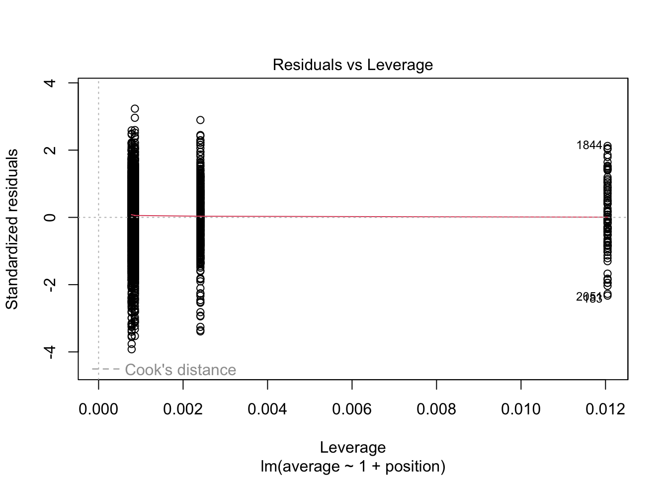
## outfield 4.974152e-17 0.8510978 0.1757679pairwise.t.test(career$average, career$position, p.adjust = 'none')$p.value[3] * (6 + 1 - 1)## [1] 2.984491e-16pairwise.t.test(career$average, career$position, p.adjust = 'none')$p.value[2] * (6 + 1 - 2)## [1] 2.516609e-13pairwise.t.test(career$average, career$position, p.adjust = 'none')$p.value[1] * (6 + 1 - 3)## [1] 0.0001152136pairwise.t.test(career$average, career$position, p.adjust = 'none')$p.value[9] * (6 + 1 - 4)## [1] 0.5273037pairwise.t.test(career$average, career$position, p.adjust = 'none')$p.value[5] * (6 + 1 - 5)## [1] 1.002638pairwise.t.test(career$average, career$position, p.adjust = 'none')$p.value[6] * (6 + 1 - 6)## [1] 0.8510978Exploring assumptions/Data Conditions for model with categorical attributes
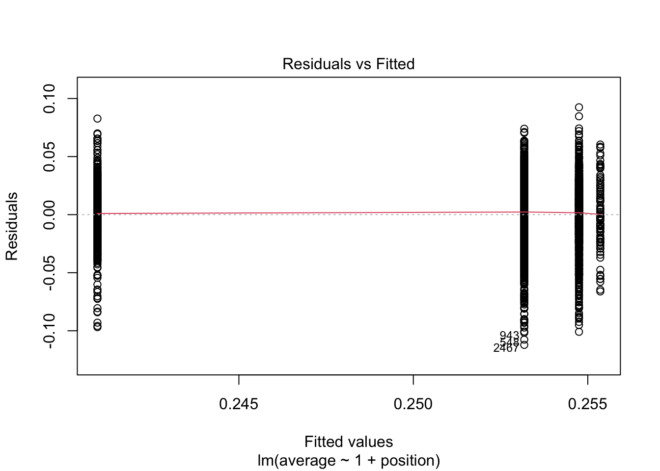
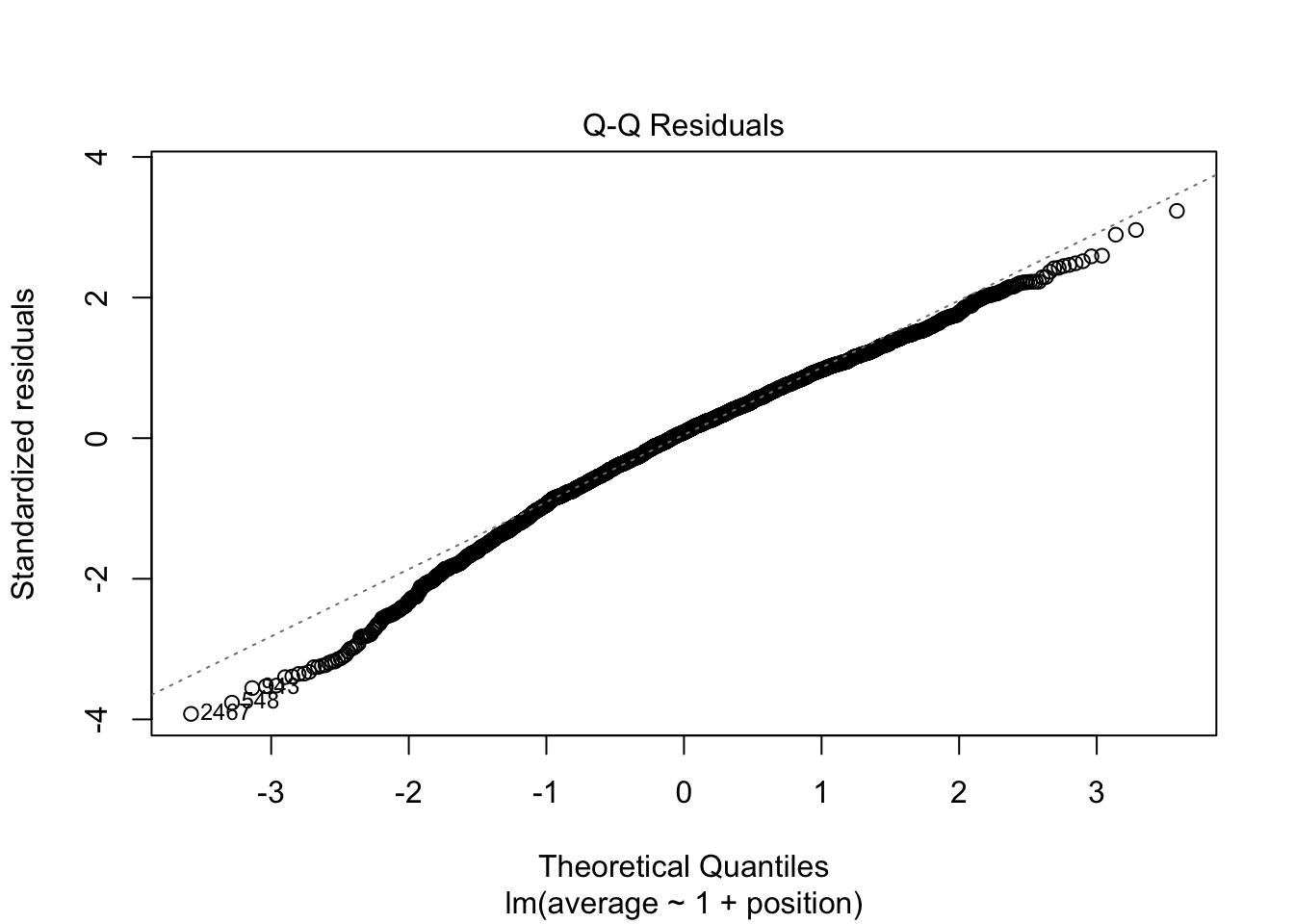
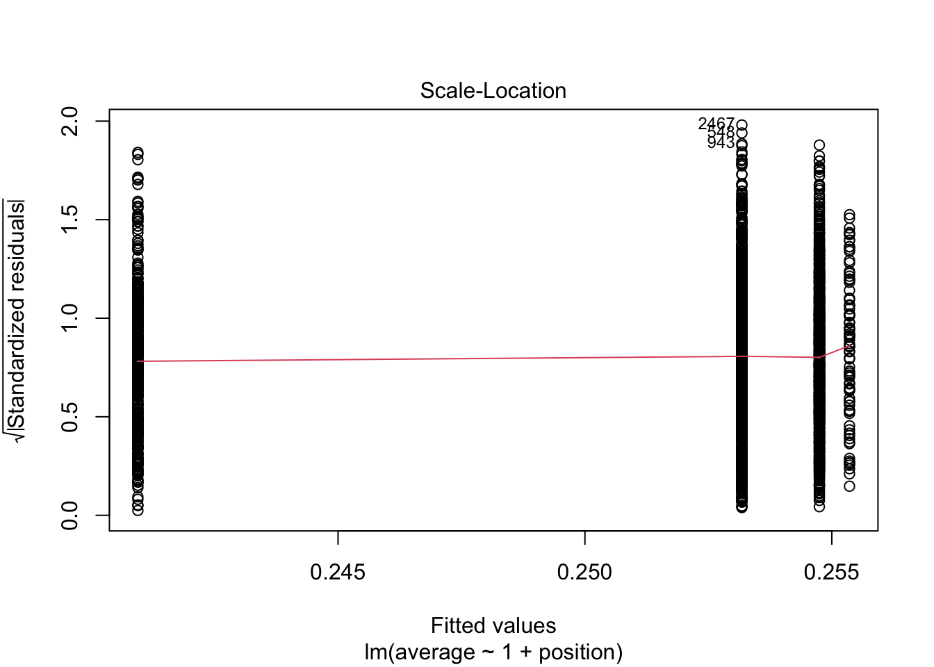
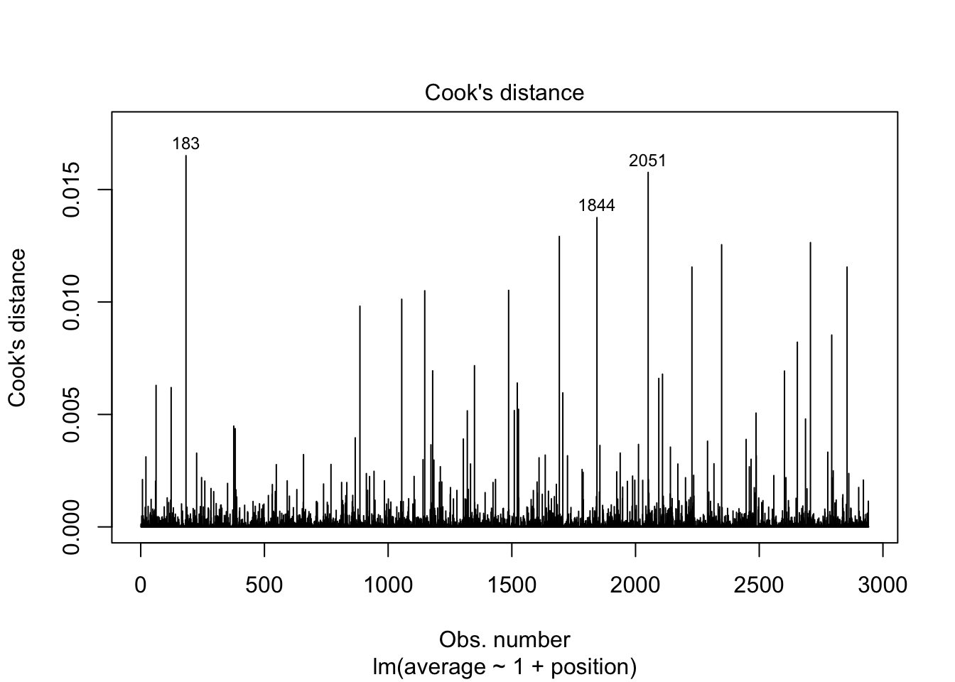
plot(position_lm, which = 1:5)