Multiple Regression
Multiple Regression
So far, the course has considered a single continuous predictor attribute. That is, in the following equation, we have only considered a single \(X\) attribute.
\[ Y = \beta_{0} + \beta_{1} X + \epsilon \]
However, there are many situations where we would want more than one predictor attribute in the data. We can simply add another predictor attribute and this would look like the following regression equation.
\[ Y = \beta_{0} + \beta_{1} X_{1} + \beta_{2} X_{2} + \epsilon \]
where \(X_{1}\) and \(X_{2}\) are two different predictors attributes. Let’s dive right into some data to explore this a bit more.
Data
For this portion, using data from the college scorecard representing information about higher education institutions.
library(tidyverse)## ── Attaching core tidyverse packages ──────────────────────── tidyverse 2.0.0 ──
## ✔ dplyr 1.1.4 ✔ readr 2.1.5
## ✔ forcats 1.0.0 ✔ stringr 1.5.1
## ✔ ggplot2 3.4.4 ✔ tibble 3.2.1
## ✔ lubridate 1.9.3 ✔ tidyr 1.3.1
## ✔ purrr 1.0.2
## ── Conflicts ────────────────────────────────────────── tidyverse_conflicts() ──
## ✖ dplyr::filter() masks stats::filter()
## ✖ dplyr::lag() masks stats::lag()
## ℹ Use the conflicted package (<http://conflicted.r-lib.org/>) to force all conflicts to become errorslibrary(ggformula)## Loading required package: scales
##
## Attaching package: 'scales'
##
## The following object is masked from 'package:purrr':
##
## discard
##
## The following object is masked from 'package:readr':
##
## col_factor
##
## Loading required package: ggridges
##
## New to ggformula? Try the tutorials:
## learnr::run_tutorial("introduction", package = "ggformula")
## learnr::run_tutorial("refining", package = "ggformula")theme_set(theme_bw(base_size = 18))
college <- read_csv("https://raw.githubusercontent.com/lebebr01/statthink/main/data-raw/College-scorecard-4143.csv")## Rows: 7058 Columns: 16
## ── Column specification ────────────────────────────────────────────────────────
## Delimiter: ","
## chr (6): instnm, city, stabbr, preddeg, region, locale
## dbl (10): adm_rate, actcmmid, ugds, costt4_a, costt4_p, tuitionfee_in, tuiti...
##
## ℹ Use `spec()` to retrieve the full column specification for this data.
## ℹ Specify the column types or set `show_col_types = FALSE` to quiet this message.head(college)## # A tibble: 6 × 16
## instnm city stabbr preddeg region locale adm_rate actcmmid ugds costt4_a
## <chr> <chr> <chr> <chr> <chr> <chr> <dbl> <dbl> <dbl> <dbl>
## 1 Alabama A… Norm… AL Bachel… South… City:… 0.903 18 4824 22886
## 2 Universit… Birm… AL Bachel… South… City:… 0.918 25 12866 24129
## 3 Amridge U… Mont… AL Bachel… South… City:… NA NA 322 15080
## 4 Universit… Hunt… AL Bachel… South… City:… 0.812 28 6917 22108
## 5 Alabama S… Mont… AL Bachel… South… City:… 0.979 18 4189 19413
## 6 The Unive… Tusc… AL Bachel… South… City:… 0.533 28 32387 28836
## # ℹ 6 more variables: costt4_p <dbl>, tuitionfee_in <dbl>,
## # tuitionfee_out <dbl>, debt_mdn <dbl>, grad_debt_mdn <dbl>, female <dbl>Question
Suppose we were interested in exploring admission rates and which attributes helped to explain variation in admission rates.
gf_density(~ adm_rate, data = college) %>%
  gf_labs(x = "Admission Rate")
## Warning: Removed 5039 rows containing non-finite values (`stat_density()`).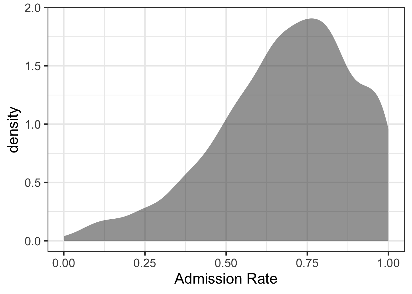
gf_point(adm_rate ~ actcmmid, data = college) %>%
  gf_smooth(method = 'loess') %>%
  gf_labs(x = "Median ACT Score",
          y = "Admission Rate")
## Warning: Removed 5769 rows containing non-finite values (`stat_smooth()`).## Warning: Removed 5769 rows containing missing values (`geom_point()`).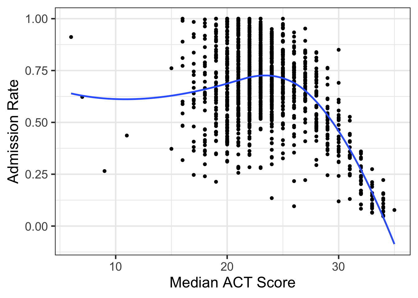
library(GGally)## Registered S3 method overwritten by 'GGally':
## method from
## +.gg ggplot2ggpairs(college[c('adm_rate', 'actcmmid', 'costt4_a')])## Warning: Removed 5039 rows containing non-finite values (`stat_density()`).## Warning in ggally_statistic(data = data, mapping = mapping, na.rm = na.rm, :
## Removed 5769 rows containing missing values## Warning in ggally_statistic(data = data, mapping = mapping, na.rm = na.rm, :
## Removed 5236 rows containing missing values## Warning: Removed 5769 rows containing missing values (`geom_point()`).## Warning: Removed 5769 rows containing non-finite values (`stat_density()`).## Warning in ggally_statistic(data = data, mapping = mapping, na.rm = na.rm, :
## Removed 5777 rows containing missing values## Warning: Removed 5236 rows containing missing values (`geom_point()`).## Warning: Removed 5777 rows containing missing values (`geom_point()`).## Warning: Removed 3486 rows containing non-finite values (`stat_density()`).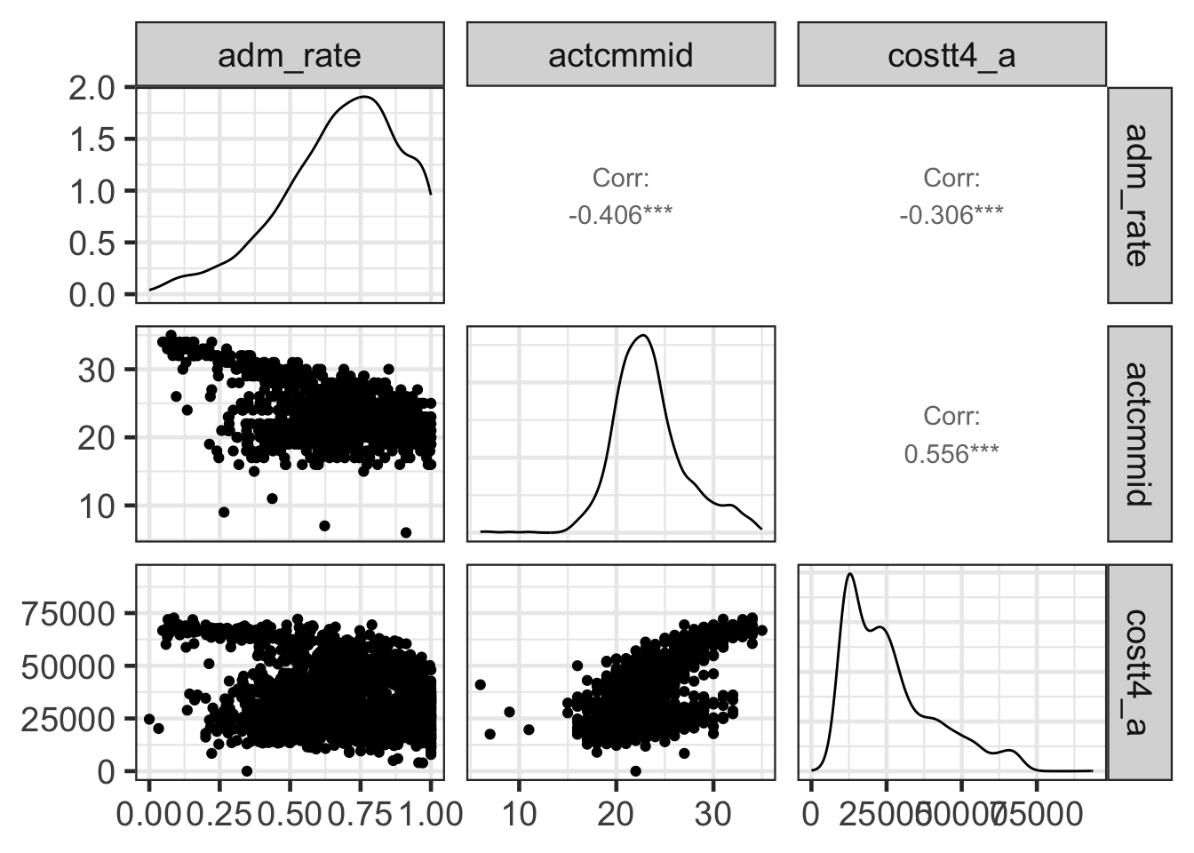
Let’s now fit a multiple regression model.
adm_mult_reg <- lm(adm_rate ~ actcmmid + costt4_a, data = college)

summary(adm_mult_reg)
##
## Call:
## lm(formula = adm_rate ~ actcmmid + costt4_a, data = college)
##
## Residuals:
## Min 1Q Median 3Q Max
## -0.65484 -0.12230 0.02291 0.13863 0.37054
##
## Coefficients:
## Estimate Std. Error t value Pr(>|t|)
## (Intercept) 1.135e+00 3.326e-02 34.130 < 2e-16 ***
## actcmmid -1.669e-02 1.650e-03 -10.114 < 2e-16 ***
## costt4_a -2.304e-06 4.047e-07 -5.693 1.55e-08 ***
## ---
## Signif. codes: 0 '***' 0.001 '**' 0.01 '*' 0.05 '.' 0.1 ' ' 1
##
## Residual standard error: 0.1813 on 1278 degrees of freedom
## (5777 observations deleted due to missingness)
## Multiple R-squared: 0.1836, Adjusted R-squared: 0.1824
## F-statistic: 143.8 on 2 and 1278 DF, p-value: < 2.2e-16This model is now the following form:
\[ Admission\ Rate = 1.1 + -0.017 ACT + -0.000002 cost + \epsilon \]
- Why are these parameter estimates so small?
- How well is the overall model doing?
- Are both terms important in understanding variation in admission rates? How can you tell?
Variance decomposition
Ultimately, multiple regression is a decomposition of variance. Recall,
\[ \sum (Y - \bar{Y})^2 = \sum (\hat{Y} - \bar{Y})^2 + \sum (Y - \hat{Y})^2 \\[10pt] SS_{Total} = SS_{Regression} + SS_{Error} \]
Multiple regression still does this, but now, there are two attributes going into helping explain variation in the regression portion of the variance decomposition. How is this variance decomposed by default? For linear regression, the variance decomposition is commonly done using type I sum of square decomposition. What does this mean? Essentially, this means that additional terms are added to determine if they help explain variation over and above the other terms in the model. This is a conditional variance added. For example, given the model above, the variance decomposition could be broken down into the following.
\[ SS_{Total} = SS_{Regression} + SS_{Error} \\[10pt] SS_{Total} = SS_{X_{1}} + SS_{X_{2} | X_{1}} + SS_{Error} \]
act_lm <- lm(adm_rate ~ actcmmid, data = college)

summary(act_lm)
##
## Call:
## lm(formula = adm_rate ~ actcmmid, data = college)
##
## Residuals:
## Min 1Q Median 3Q Max
## -0.71615 -0.12521 0.02024 0.14490 0.37314
##
## Coefficients:
## Estimate Std. Error t value Pr(>|t|)
## (Intercept) 1.180914 0.032988 35.80 <2e-16 ***
## actcmmid -0.022162 0.001391 -15.93 <2e-16 ***
## ---
## Signif. codes: 0 '***' 0.001 '**' 0.01 '*' 0.05 '.' 0.1 ' ' 1
##
## Residual standard error: 0.1844 on 1287 degrees of freedom
## (5769 observations deleted due to missingness)
## Multiple R-squared: 0.1647, Adjusted R-squared: 0.1641
## F-statistic: 253.8 on 1 and 1287 DF, p-value: < 2.2e-16anova(act_lm)## Analysis of Variance Table
##
## Response: adm_rate
## Df Sum Sq Mean Sq F value Pr(>F)
## actcmmid 1 8.635 8.6351 253.84 < 2.2e-16 ***
## Residuals 1287 43.781 0.0340
## ---
## Signif. codes: 0 '***' 0.001 '**' 0.01 '*' 0.05 '.' 0.1 ' ' 1anova(adm_mult_reg)## Analysis of Variance Table
##
## Response: adm_rate
## Df Sum Sq Mean Sq F value Pr(>F)
## actcmmid 1 8.386 8.3861 255.092 < 2.2e-16 ***
## costt4_a 1 1.065 1.0655 32.411 1.546e-08 ***
## Residuals 1278 42.014 0.0329
## ---
## Signif. codes: 0 '***' 0.001 '**' 0.01 '*' 0.05 '.' 0.1 ' ' 1cost_lm <- lm(adm_rate ~ costt4_a, data = college)
summary(cost_lm)##
## Call:
## lm(formula = adm_rate ~ costt4_a, data = college)
##
## Residuals:
## Min 1Q Median 3Q Max
## -0.72108 -0.12656 0.02474 0.14459 0.38059
##
## Coefficients:
## Estimate Std. Error t value Pr(>|t|)
## (Intercept) 8.233e-01 1.151e-02 71.52 <2e-16 ***
## costt4_a -4.147e-06 3.022e-07 -13.73 <2e-16 ***
## ---
## Signif. codes: 0 '***' 0.001 '**' 0.01 '*' 0.05 '.' 0.1 ' ' 1
##
## Residual standard error: 0.1965 on 1820 degrees of freedom
## (5236 observations deleted due to missingness)
## Multiple R-squared: 0.0938, Adjusted R-squared: 0.09331
## F-statistic: 188.4 on 1 and 1820 DF, p-value: < 2.2e-16anova(cost_lm)## Analysis of Variance Table
##
## Response: adm_rate
## Df Sum Sq Mean Sq F value Pr(>F)
## costt4_a 1 7.278 7.2781 188.4 < 2.2e-16 ***
## Residuals 1820 70.309 0.0386
## ---
## Signif. codes: 0 '***' 0.001 '**' 0.01 '*' 0.05 '.' 0.1 ' ' 1