Linear Regression Data Conditions

Conditions for Linear Regression

The conditions surrounding linear regression typically surround the residuals. Residuals are defined as:

\[ Y - \hat{Y} \]

These are the deviations in the observed scores from the predicted scores from the linear regression. Recall, through least square estimation that these residauls will sum to 0, therefore, their mean would also be equal to 0. However, there are certain conditions about these residuals that are made for the linear regression model to have the inferences be appropriate. We’ll talk more about what the implications for violating these conditions will have on the linear regression model, but first, the conditions.

Approximately Normally distributed residuals
Homogeneity of variance
Uncorrelated residuals
Error term is uncorrelated with the predictor attribute
Linearity and additivity of the model.

Each of these will be discussed in turn.

Data conditions that are not directly testable:

Validity
Representativeness

Data

The data for this section of notes will explore data from the Environmental Protection Agency on Air Quality collected for the state of Iowa in 2021. The data are daily values for PM 2.5 particulates. The attributes included in the data are shown below with a short description.

Variable	Description
date	Date of observation
id	Site ID
poc	Parameter Occurrence Code (POC)
pm2.5	Average daily pm 2.5 particulate value, in (ug/m3; micrograms per meter cubed)
daily_aqi	Average air quality index
site_name	Site Name
aqs_parameter_desc	Text Description of Observation
cbsa_code	Core Based Statistical Area (CBSA) ID
cbsa_name	CBSA Name
county	County in Iowa
avg_wind	Average daily wind speed (in knots)
max_wind	Maximum daily wind speed (in knots)
max_wind_hours	Time of maximum daily wind speed

Guiding Question

How is average daily wind speed related to the daily air quality index?

library(tidyverse)

## ── Attaching core tidyverse packages ──────────────────────── tidyverse 2.0.0 ──
## ✔ dplyr     1.1.4     ✔ readr     2.1.5
## ✔ forcats   1.0.0     ✔ stringr   1.5.1
## ✔ ggplot2   3.4.4     ✔ tibble    3.2.1
## ✔ lubridate 1.9.3     ✔ tidyr     1.3.1
## ✔ purrr     1.0.2     
## ── Conflicts ────────────────────────────────────────── tidyverse_conflicts() ──
## ✖ dplyr::filter() masks stats::filter()
## ✖ dplyr::lag()    masks stats::lag()
## ℹ Use the conflicted package (<http://conflicted.r-lib.org/>) to force all conflicts to become errors

library(ggformula)

## Loading required package: scales
## 
## Attaching package: 'scales'
## 
## The following object is masked from 'package:purrr':
## 
##     discard
## 
## The following object is masked from 'package:readr':
## 
##     col_factor
## 
## Loading required package: ggridges
## 
## New to ggformula?  Try the tutorials: 
## 	learnr::run_tutorial("introduction", package = "ggformula")
## 	learnr::run_tutorial("refining", package = "ggformula")

library(mosaic)

## Registered S3 method overwritten by 'mosaic':
##   method                           from   
##   fortify.SpatialPolygonsDataFrame ggplot2
## 
## The 'mosaic' package masks several functions from core packages in order to add 
## additional features.  The original behavior of these functions should not be affected by this.
## 
## Attaching package: 'mosaic'
## 
## The following object is masked from 'package:Matrix':
## 
##     mean
## 
## The following object is masked from 'package:scales':
## 
##     rescale
## 
## The following objects are masked from 'package:dplyr':
## 
##     count, do, tally
## 
## The following object is masked from 'package:purrr':
## 
##     cross
## 
## The following object is masked from 'package:ggplot2':
## 
##     stat
## 
## The following objects are masked from 'package:stats':
## 
##     binom.test, cor, cor.test, cov, fivenum, IQR, median, prop.test,
##     quantile, sd, t.test, var
## 
## The following objects are masked from 'package:base':
## 
##     max, mean, min, prod, range, sample, sum

theme_set(theme_bw(base_size = 18))

airquality <- readr::read_csv("https://raw.githubusercontent.com/lebebr01/psqf_6243/main/data/iowa_air_quality_2021.csv")

## Rows: 6917 Columns: 10
## ── Column specification ────────────────────────────────────────────────────────
## Delimiter: ","
## chr (5): date, site_name, aqs_parameter_desc, cbsa_name, county
## dbl (5): id, poc, pm2.5, daily_aqi, cbsa_code
## 
## ℹ Use `spec()` to retrieve the full column specification for this data.
## ℹ Specify the column types or set `show_col_types = FALSE` to quiet this message.

wind <- readr::read_csv("https://raw.githubusercontent.com/lebebr01/psqf_6243/main/data/daily_WIND_2021-iowa.csv")

## Rows: 1537 Columns: 5
## ── Column specification ────────────────────────────────────────────────────────
## Delimiter: ","
## chr (2): date, cbsa_name
## dbl (3): avg_wind, max_wind, max_wind_hours
## 
## ℹ Use `spec()` to retrieve the full column specification for this data.
## ℹ Specify the column types or set `show_col_types = FALSE` to quiet this message.

airquality <- airquality |>
   left_join(wind, by = c('cbsa_name', 'date')) |> 
   drop_na()

## Warning in left_join(airquality, wind, by = c("cbsa_name", "date")): Detected an unexpected many-to-many relationship between `x` and `y`.
## ℹ Row 21 of `x` matches multiple rows in `y`.
## ℹ Row 1 of `y` matches multiple rows in `x`.
## ℹ If a many-to-many relationship is expected, set `relationship =
##   "many-to-many"` to silence this warning.

air_lm <- lm(daily_aqi ~ avg_wind, data = airquality)
coef(air_lm)

## (Intercept)    avg_wind 
##   48.222946   -2.211798

The residuals can be saved with the resid() function. These can also be added to the original data, which are particularly helpful.

head(resid(air_lm))

##          1          2          3          4          5          6 
##  15.283427  11.186742  25.191433  15.398540   8.246896 -12.749410

airquality$residuals <- resid(air_lm)
head(airquality)

## # A tibble: 6 × 14
##   date           id   poc pm2.5 daily_aqi site_name aqs_parameter_desc cbsa_code
##   <chr>       <dbl> <dbl> <dbl>     <dbl> <chr>     <chr>                  <dbl>
## 1 1/1/21  190130009     1  15.1        57 Water To… PM2.5 - Local Con…     47940
## 2 1/4/21  190130009     1  13.3        54 Water To… PM2.5 - Local Con…     47940
## 3 1/7/21  190130009     1  20.5        69 Water To… PM2.5 - Local Con…     47940
## 4 1/10/21 190130009     1  14.3        56 Water To… PM2.5 - Local Con…     47940
## 5 1/13/21 190130009     1  13.7        54 Water To… PM2.5 - Local Con…     47940
## 6 1/16/21 190130009     1   5.3        22 Water To… PM2.5 - Local Con…     47940
## # ℹ 6 more variables: cbsa_name <chr>, county <chr>, avg_wind <dbl>,
## #   max_wind <dbl>, max_wind_hours <dbl>, residuals <dbl>

Approximately Normally distributed residuals

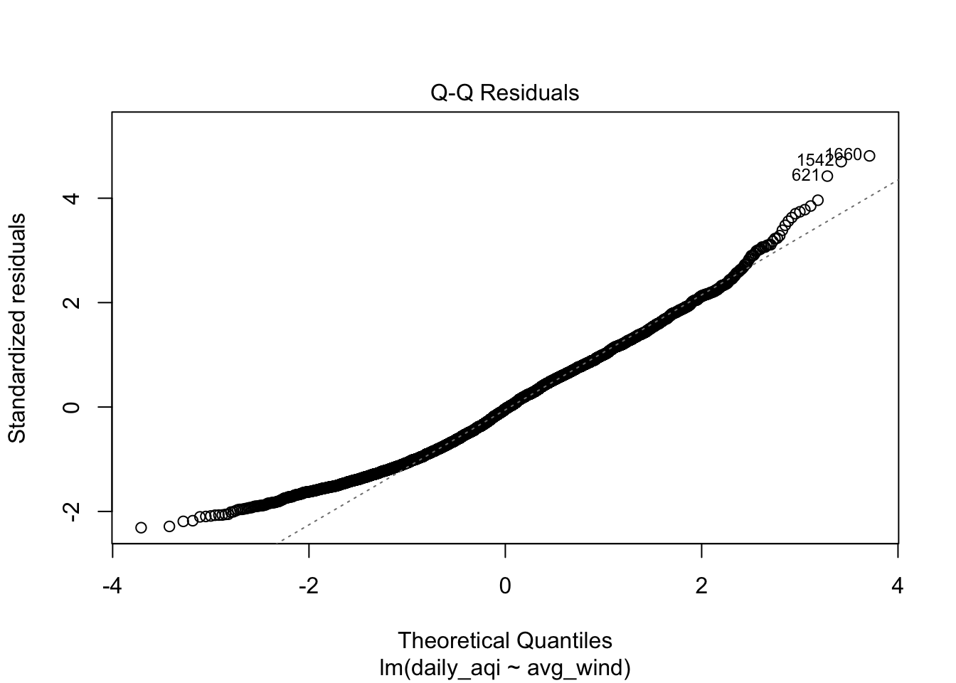
The first assumption is that the residuals are at least approximately Normally distributed. This assumption is really only much of a concern when the sample size is small. If the sample size is larger, the Central Limit Thereom (CLT) states that the distribution of the statstics will be approximately normally distributed. The threshold for the CLT to be properly invoked is about 30. Larger then this, the residuals do not need to be approximately normally distributed. Even still, exploring the distribution of the residuals can still be helpful and can also be helpful to identify potential extreme values.

This example will make use of the air quality data one more time.

gf_density(~ residuals, data = airquality) |>
  gf_labs(x = "Residuals")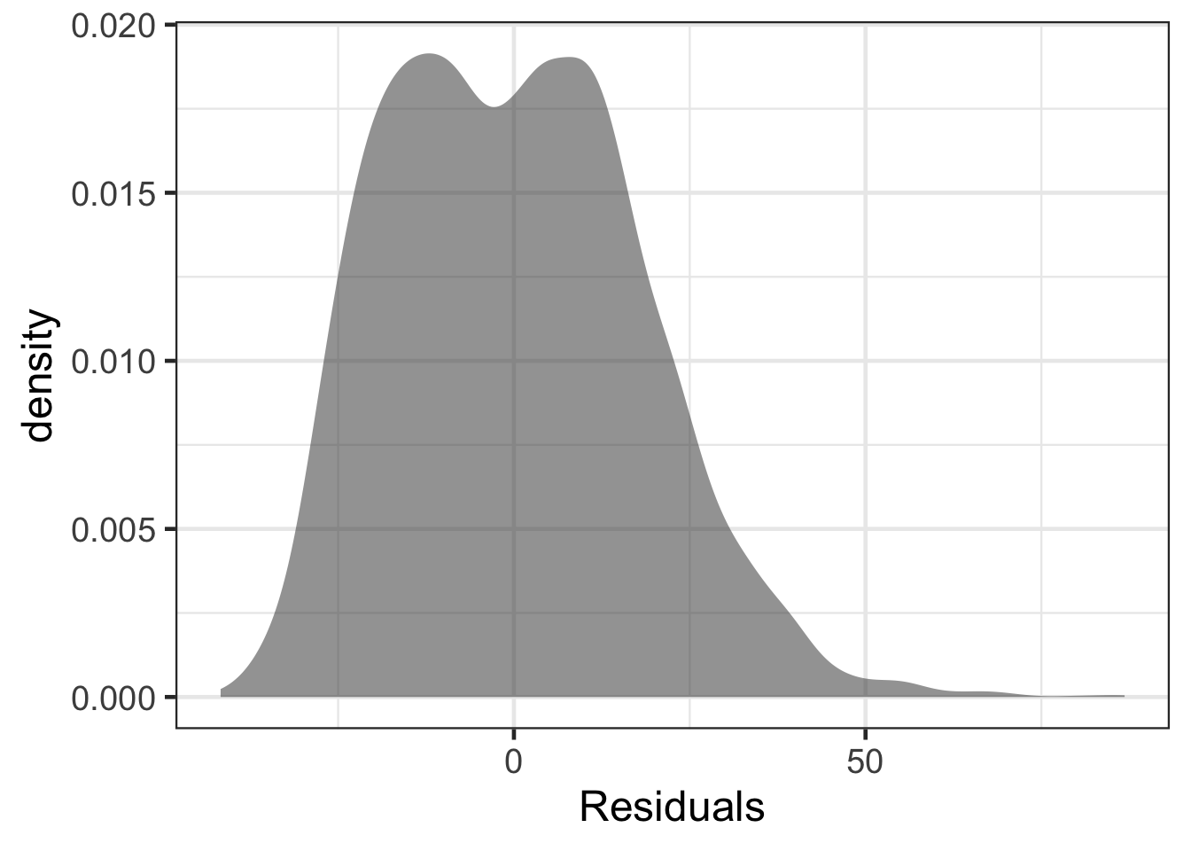

ggplot(airquality, aes(sample = residuals)) + 
  stat_qq(size = 5) + 
  stat_qq_line(linewidth = 2)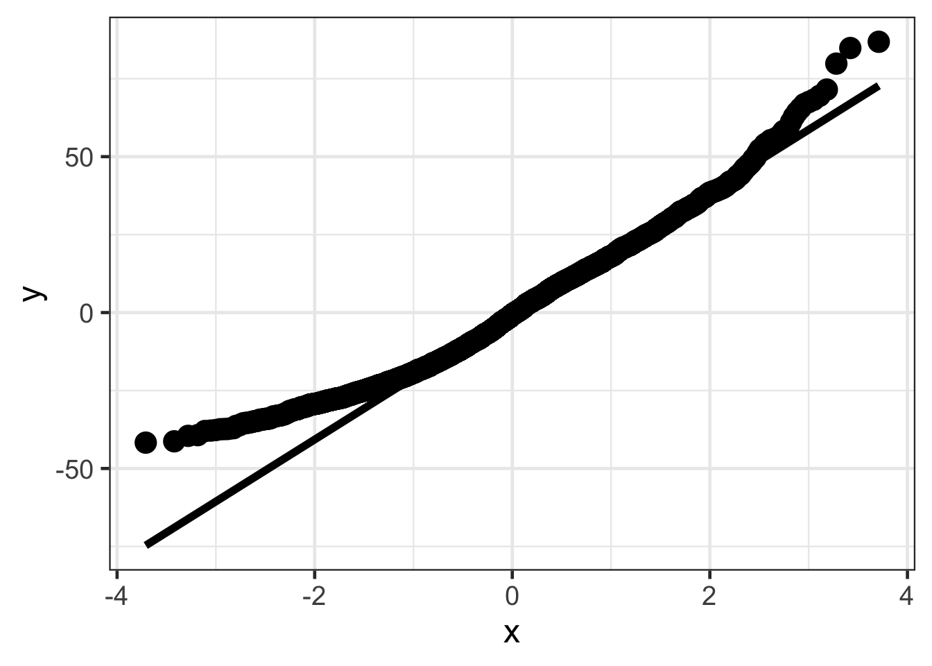

Different QQ plots by distribution type

This next section will generate some residuals that would fit certain types you may see in practice. These are meant as a way to give you some data from residuals that would be common in practice.

Symmetric / Normally Distributed Residuals

# install.packages('patchwork')
library(patchwork)

sim_resid <- data.frame(residuals = rnorm(500, 0, sd = 1))

dens <- gf_density(~ residuals, data = sim_resid) |>
  gf_labs(x = "Residuals")

qq_plot <- ggplot(sim_resid, aes(sample = residuals)) + 
  stat_qq(size = 5) + 
  stat_qq_line(linewidth = 2)

dens + qq_plot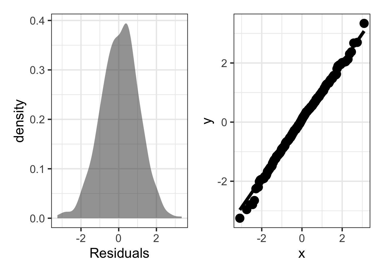

Skewed Residuals

sim_resid <- data.frame(residuals = rchisq(500, df = 1) - 1)

dens <- gf_density(~ residuals, data = sim_resid) |>
  gf_labs(x = "Residuals")

qq_plot <- ggplot(sim_resid, aes(sample = residuals)) + 
  stat_qq(size = 5) + 
  stat_qq_line(linewidth = 2)

dens + qq_plot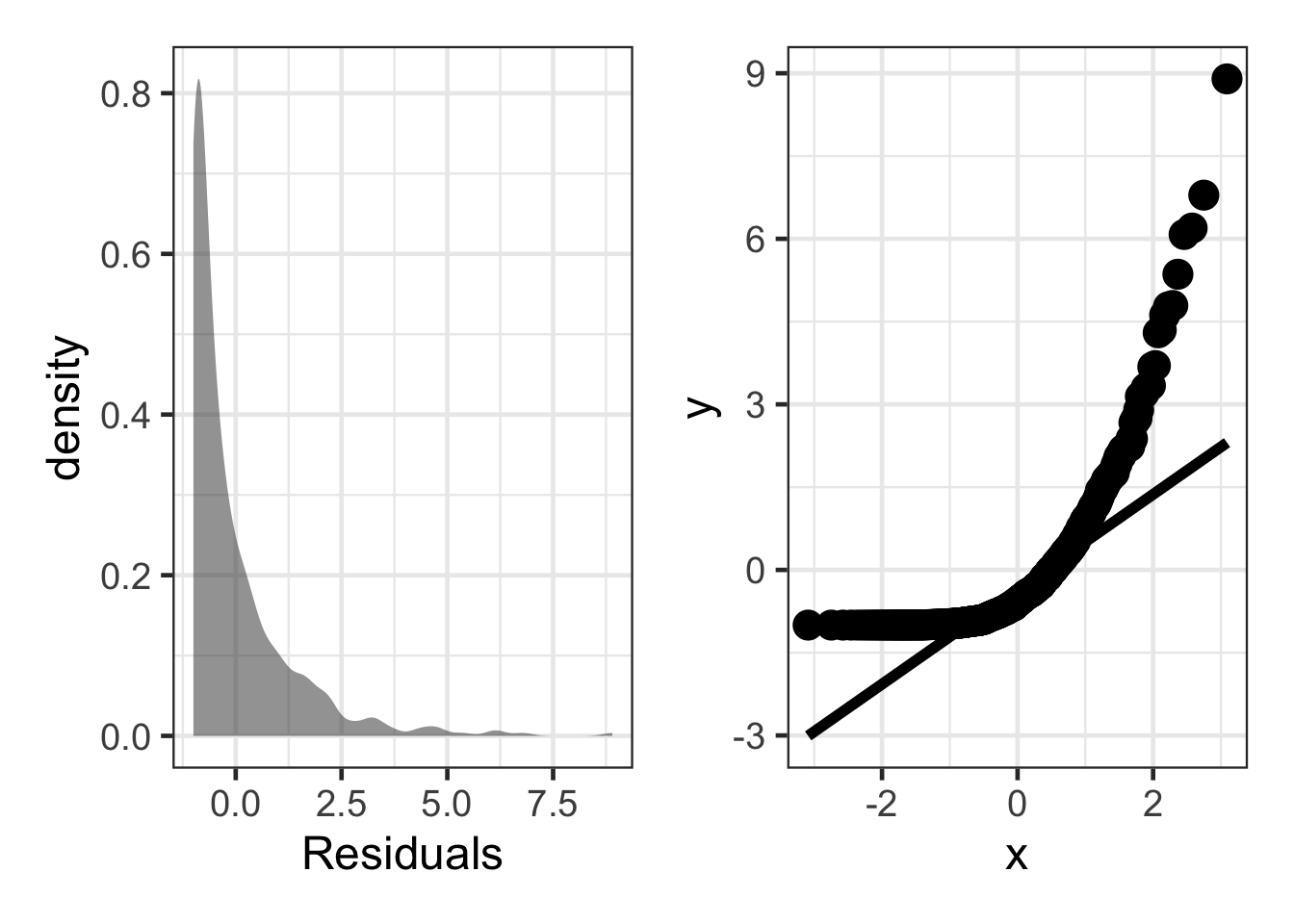

Negatively Skewed

sim_resid <- data.frame(residuals = (rchisq(500, df = 1) - 1) * -1)

dens <- gf_density(~ residuals, data = sim_resid) |>
  gf_labs(x = "Residuals")

qq_plot <- ggplot(sim_resid, aes(sample = residuals)) + 
  stat_qq(size = 5) + 
  stat_qq_line(linewidth = 2)

dens + qq_plot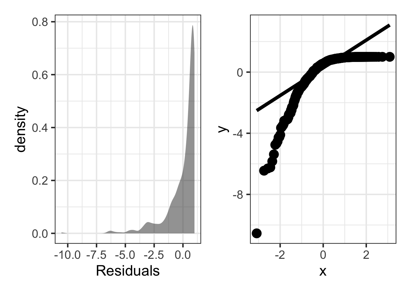

Heavy Tails

sim_resid <- data.frame(residuals = (rt(500, df = 4)))

dens <- gf_density(~ residuals, data = sim_resid) |>
  gf_labs(x = "Residuals")

qq_plot <- ggplot(sim_resid, aes(sample = residuals)) + 
  stat_qq(size = 5) + 
  stat_qq_line(linewidth = 2)

dens + qq_plot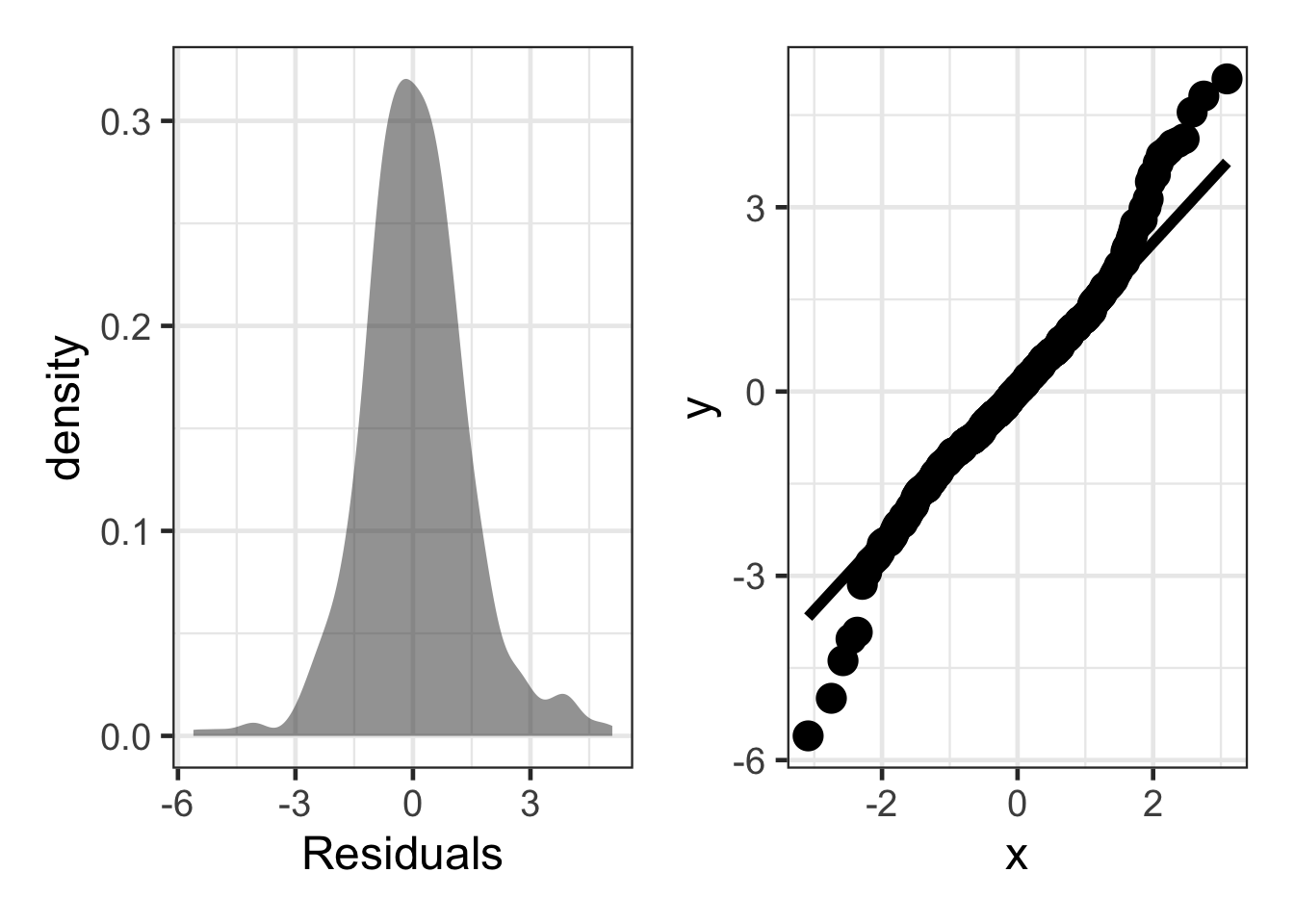

Uniform Distribution

sim_resid <- data.frame(residuals = (runif(500, min = -1, max = 1)))

dens <- gf_density(~ residuals, data = sim_resid) |>
  gf_labs(x = "Residuals")

qq_plot <- ggplot(sim_resid, aes(sample = residuals)) + 
  stat_qq(size = 5) + 
  stat_qq_line(linewidth = 2)

dens + qq_plot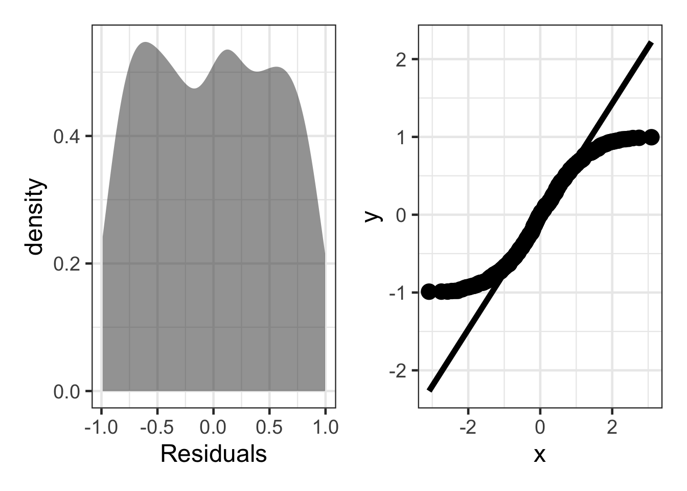

Floor Effect

sim_resid <- data.frame(residuals = (rnorm(500, mean = 0, sd = 1))) |> 
   mutate(residuals = ifelse(residuals < -1.5, -1.5, residuals))

dens <- gf_density(~ residuals, data = sim_resid) |>
  gf_labs(x = "Residuals")

qq_plot <- ggplot(sim_resid, aes(sample = residuals)) + 
  stat_qq(size = 5) + 
  stat_qq_line(linewidth = 2)

dens + qq_plot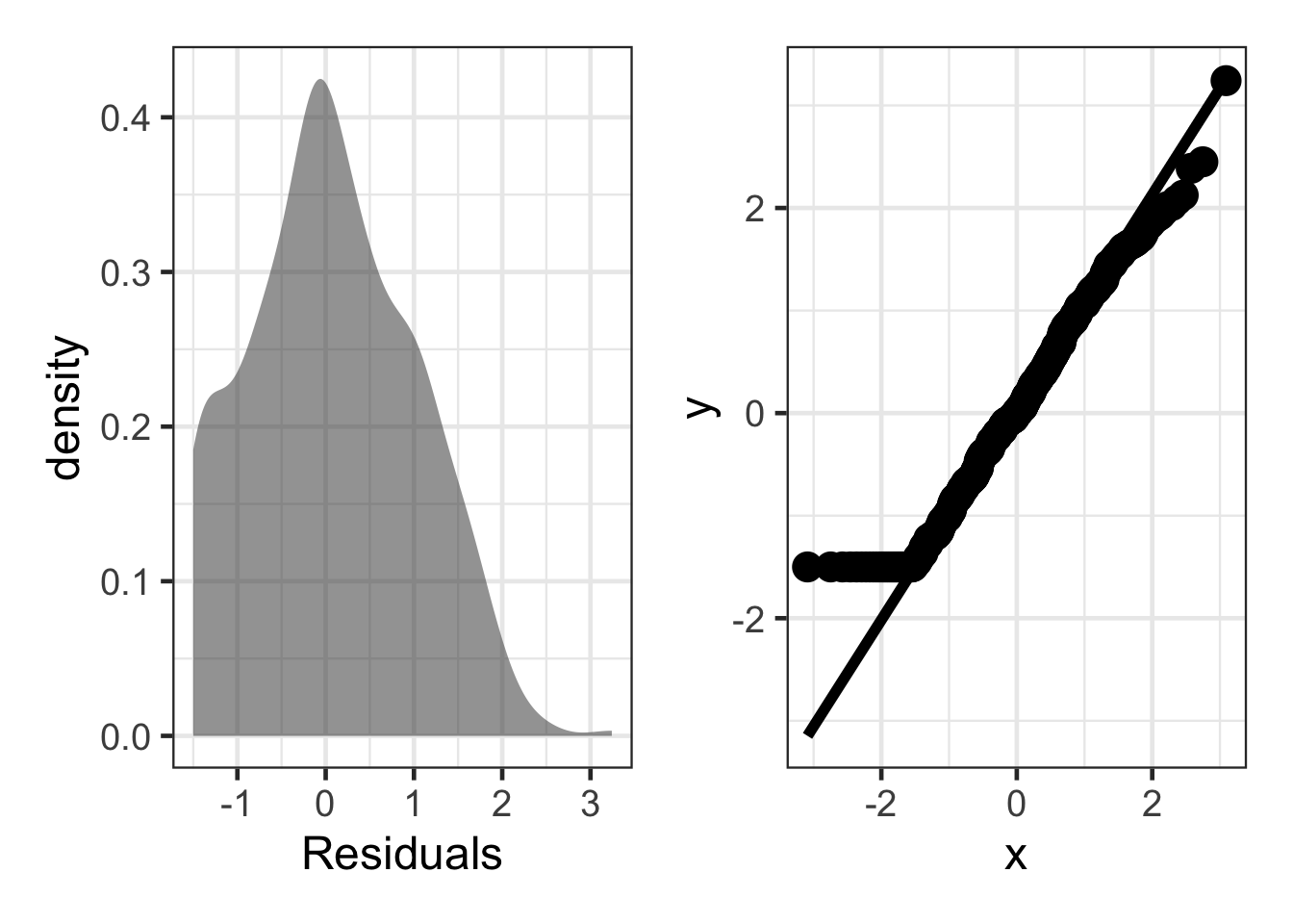

Ceiling Effect

sim_resid <- data.frame(residuals = (rnorm(500, mean = 0, sd = 1))) |> 
   mutate(residuals = ifelse(residuals > 1.5, 1.5, residuals))

dens <- gf_density(~ residuals, data = sim_resid) |>
  gf_labs(x = "Residuals")

qq_plot <- ggplot(sim_resid, aes(sample = residuals)) + 
  stat_qq(size = 5) + 
  stat_qq_line(linewidth = 2)

dens + qq_plot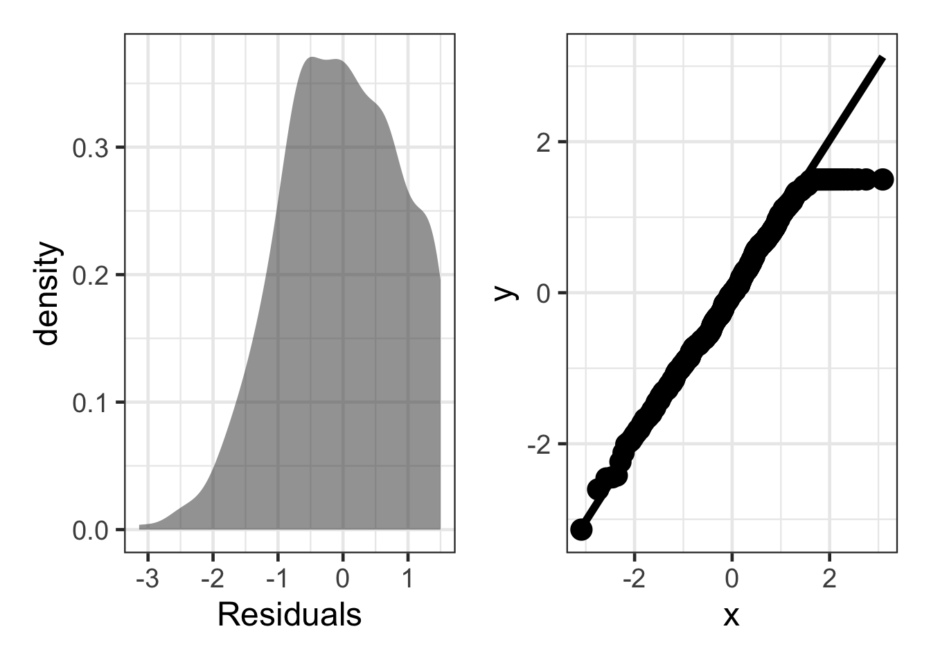

Standardized Residuals

Standardized residuals can be another way to explore the residuals. These will now be standardized to have a variance of 1, similar to that of a Z-score. These can be computed as:

\[ standardized\ residuals = \frac{\epsilon_{i}}{SD_{\epsilon}} \]

Within R, these can be computed using the function rstandard(). Furthermore, these can be computed from another package called broom with the augment() function.

head(rstandard(air_lm))

##          1          2          3          4          5          6 
##  0.8466153  0.6196983  1.3955421  0.8529766  0.4568937 -0.7062638

library(broom)

resid_diagnostics <- augment(air_lm)
head(resid_diagnostics)

## # A tibble: 6 × 8
##   daily_aqi avg_wind .fitted .resid     .hat .sigma   .cooksd .std.resid
##       <dbl>    <dbl>   <dbl>  <dbl>    <dbl>  <dbl>     <dbl>      <dbl>
## 1        57     2.94    41.7  15.3  0.000266   18.1 0.0000953      0.847
## 2        54     2.45    42.8  11.2  0.000318   18.1 0.0000611      0.620
## 3        69     2.00    43.8  25.2  0.000380   18.1 0.000370       1.40 
## 4        56     3.45    40.6  15.4  0.000230   18.1 0.0000836      0.853
## 5        54     1.12    45.8   8.25 0.000539   18.1 0.0000563      0.457
## 6        22     6.09    34.7 -12.7  0.000319   18.1 0.0000795     -0.706

gf_density(~ .std.resid, data = resid_diagnostics) |>
  gf_labs(x = "Standardized Residuals")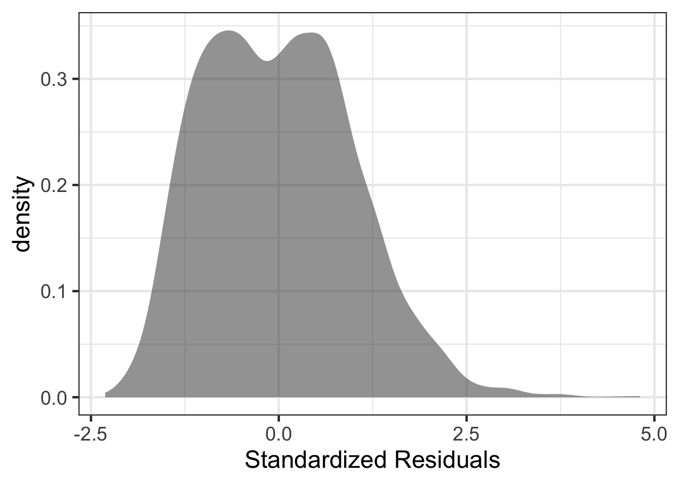

ggplot(resid_diagnostics, aes(sample = .std.resid)) + 
  stat_qq(size = 5) + 
  stat_qq_line(size = 2)

## Warning: Using `size` aesthetic for lines was deprecated in ggplot2 3.4.0.
## ℹ Please use `linewidth` instead.
## This warning is displayed once every 8 hours.
## Call `lifecycle::last_lifecycle_warnings()` to see where this warning was
## generated.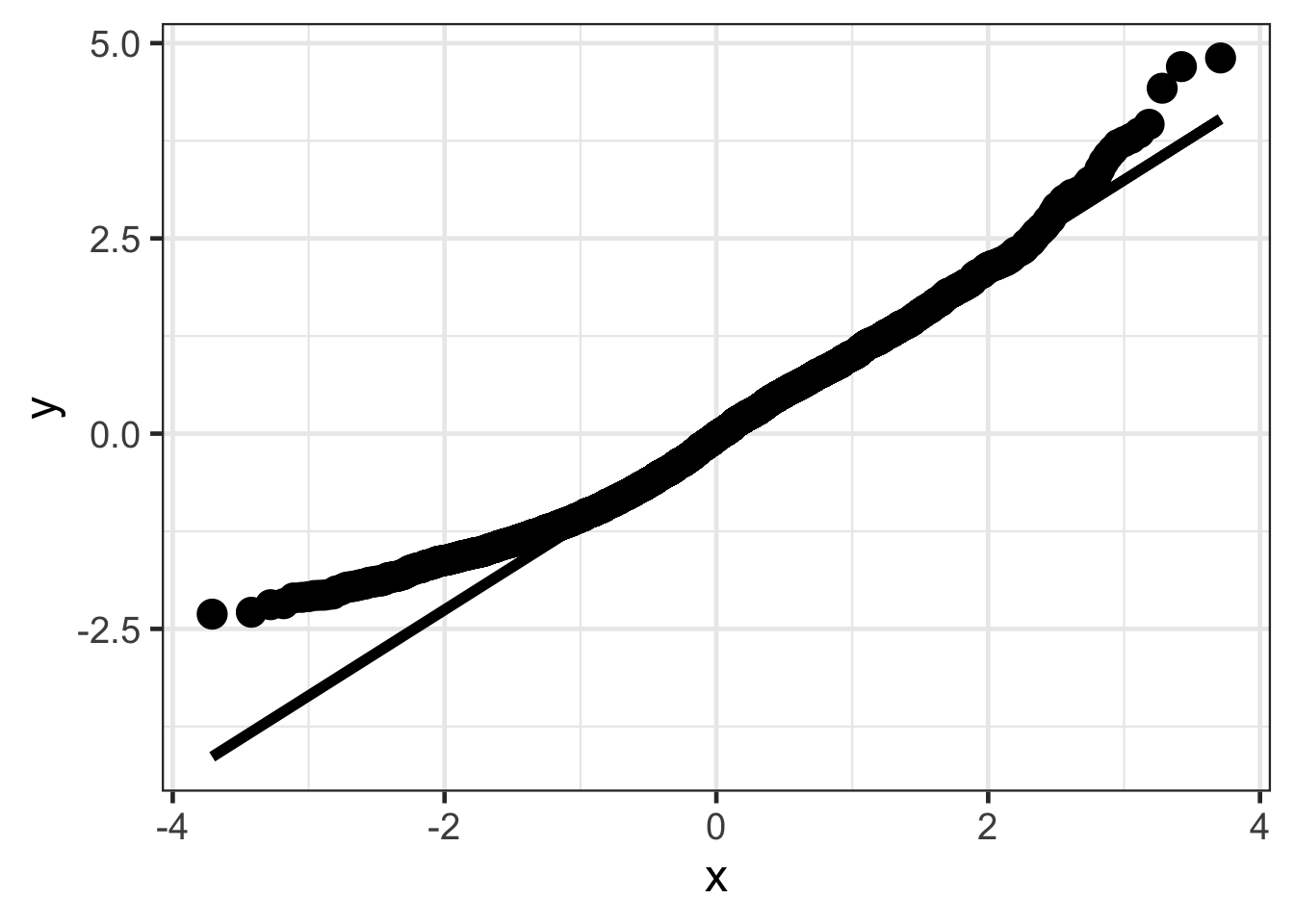

Homogeneity of variance

Homoegeneity of variance is an assumption that is of larger concern compared to normality of the residuals. Homoogeneity of variance is an assumption that states that the variance of the residuals are similar across the predicted or fitted values from the regression line. This assumption can be explored by looking at the residuals (standardized or raw residuals), by the fitted or predicted values. Within this plot, the range of residuals should be similar across the range of fitted or predicted values.

gf_point(.resid ~ .fitted, data = resid_diagnostics, size = 5, alpha = .15) |>
  gf_smooth(method = 'loess', size = 2) |>
  gf_labs(x = 'Fitted Values',
          y = 'Residuals')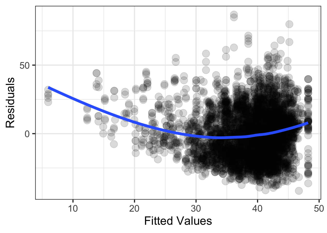

gf_point(.std.resid ~ .fitted, data = resid_diagnostics, size = 5, alpha = .15) |>
  gf_smooth(method = 'loess', size = 2) |>
  gf_labs(x = 'Fitted Values',
          y = 'Standardized Residuals')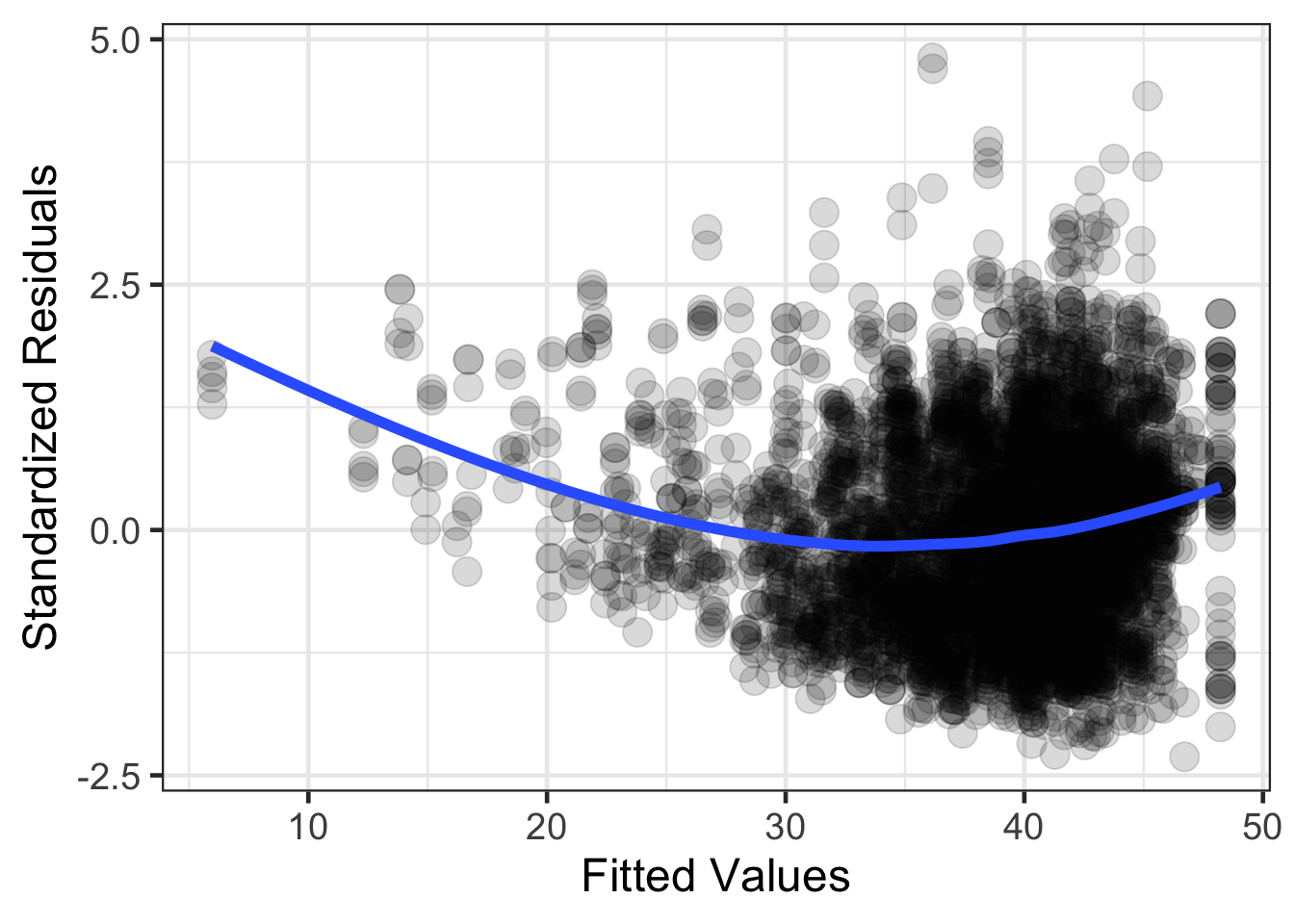

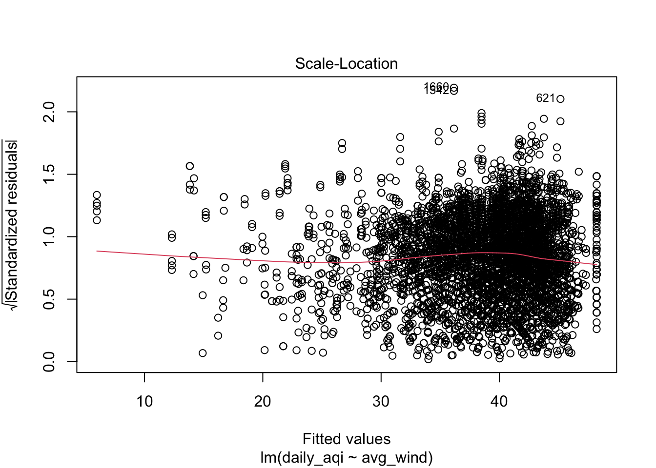
Another figure that can also be helpful for the homogeneity of variance assumption is one that rescales the residuals on the y-axis. The rescaling makes all the standardized residuals positive (takes the absolute value) and then takes the square root of this.

resid_diagnostics |>
  mutate(sqrt_abs_sresid = sqrt(abs(.std.resid))) |>
  gf_point(sqrt_abs_sresid ~ .fitted, size = 5, alpha = .15) |>
  gf_smooth(method = 'loess', size = 2) |>
  gf_labs(x = 'Fitted Values',
          y = 'Sqrt Abs Standardized Residuals')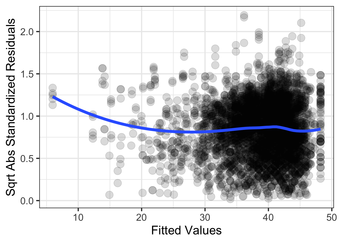

Statistical test for homogeneity of variance

There are also statistical tests that can aid in the assessing if the data are constant or not. The one that has been shown to perform relatively well is the Breusch-Pagan test. The details of the statistical test are not going to be discussed here, but we will focus on interpreting the output.

# install.packages("car")
library(car)

## Loading required package: carData

## 
## Attaching package: 'car'

## The following objects are masked from 'package:mosaic':
## 
##     deltaMethod, logit

## The following object is masked from 'package:dplyr':
## 
##     recode

## The following object is masked from 'package:purrr':
## 
##     some

air_lm <- lm(daily_aqi ~ avg_wind, data = airquality)

ncvTest(air_lm)

## Non-constant Variance Score Test 
## Variance formula: ~ fitted.values 
## Chisquare = 0.007804568, Df = 1, p = 0.9296

Data with high leverage

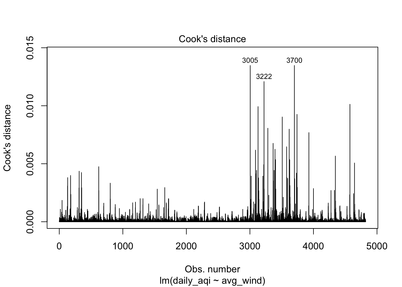
Data with high leverage are extreme values that may significantly impact the regression estimates. These statistics include extreme values for the outcome or predictor attributes. Cook’s distance is one statistic that can help to identify points with high impact/leverage for the regression estimates. Cook’s distance is a statistic that represents how much change there would be in the fitted values if the point was removed when estimating the regression coefficients. There is some disagreement between what type of thresholds to use for Cook’s distance, but one rule of thumb is Cook’s distance greater than 1. There has also been some research showing that Cook’s distance follows an F-distribution, so a more specific value could be computed. The rule of thumb for greater than 1 comes from the F distribution for large samples.

resid_diagnostics |>
  mutate(obs_num = 1:n()) |>
  gf_col(.cooksd ~ obs_num, fill = 'black', color = 'black') |>
  gf_labs(x = "Observation Number",
          y = "Cook's Distance")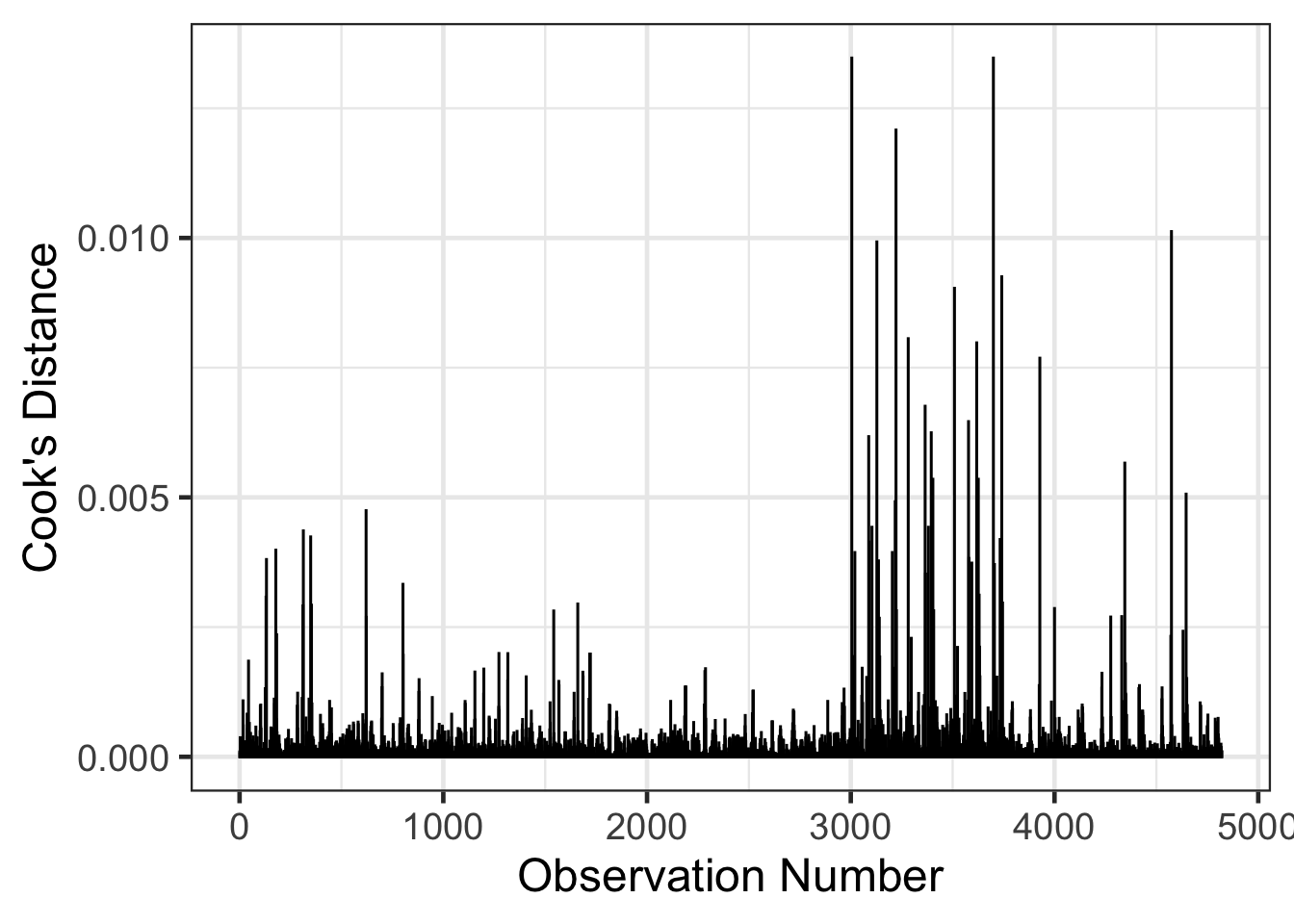

Another leave one out statistic is the studentized deleted residuals. These are computed by removing a data point, refitting the regression model, then generate a predicted value for the X value for the data point removed. Then the residual is computed the same as before and is standardized like the standardized residuals above. The function in R to compute these is rstudent().

head(rstudent(air_lm))

##          1          2          3          4          5          6 
##  0.8465904  0.6196587  1.3956793  0.8529524  0.4568561 -0.7062271

airquality$student_residuals <- rstudent(air_lm)
head(airquality)

## # A tibble: 6 × 15
##   date           id   poc pm2.5 daily_aqi site_name aqs_parameter_desc cbsa_code
##   <chr>       <dbl> <dbl> <dbl>     <dbl> <chr>     <chr>                  <dbl>
## 1 1/1/21  190130009     1  15.1        57 Water To… PM2.5 - Local Con…     47940
## 2 1/4/21  190130009     1  13.3        54 Water To… PM2.5 - Local Con…     47940
## 3 1/7/21  190130009     1  20.5        69 Water To… PM2.5 - Local Con…     47940
## 4 1/10/21 190130009     1  14.3        56 Water To… PM2.5 - Local Con…     47940
## 5 1/13/21 190130009     1  13.7        54 Water To… PM2.5 - Local Con…     47940
## 6 1/16/21 190130009     1   5.3        22 Water To… PM2.5 - Local Con…     47940
## # ℹ 7 more variables: cbsa_name <chr>, county <chr>, avg_wind <dbl>,
## #   max_wind <dbl>, max_wind_hours <dbl>, residuals <dbl>,
## #   student_residuals <dbl>

airquality |>
  mutate(obs_num = 1:n()) |>
  gf_point(student_residuals ~ obs_num, size = 5, alpha = .15) |>
  gf_hline(yintercept = ~ 3, color = 'blue', size = 2) |>
  gf_labs(x = "Observation Number",
          y = "Studentized Residuals")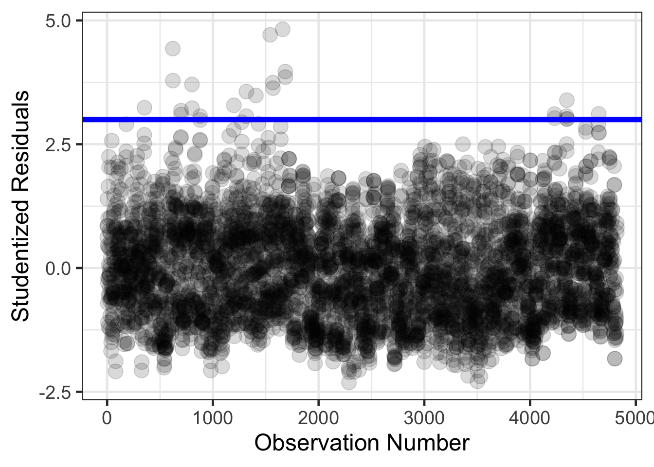

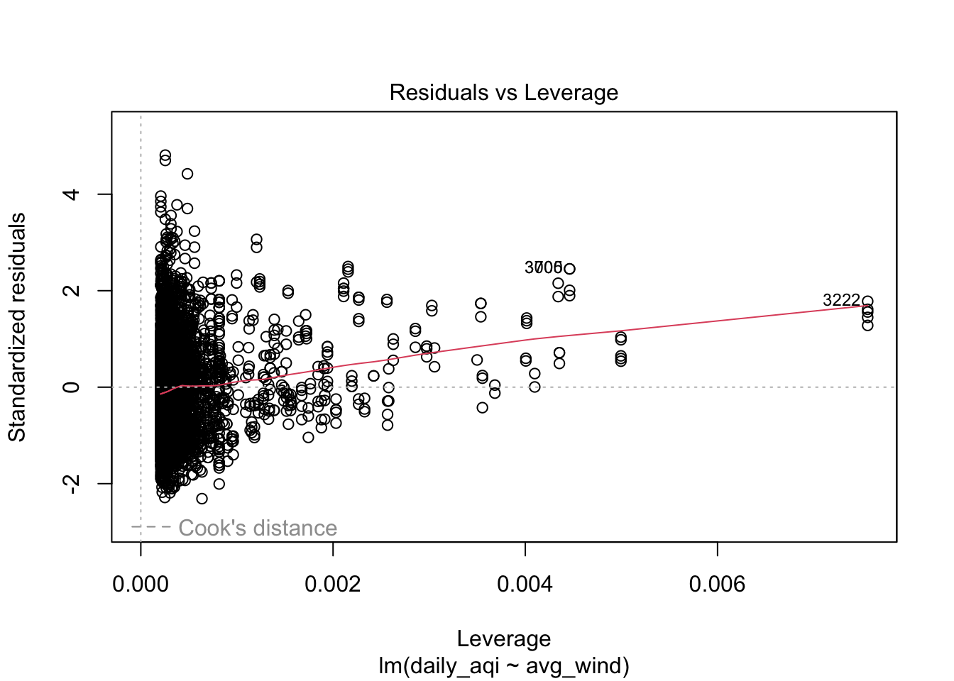
Leverage can be another measure to help detect outliers in X values. The hat values that were computed from the augment() function above and can be interpreted as the distance the X scores are from the center of all X predictors. In the case of a single predictor, the hat values are the distance the X score is from the mean of X. The hat values will also sum up to the number of predictors and will always range between 0 and 1.

resid_diagnostics |>
  mutate(obs_num = 1:n()) |>
  gf_col(.hat ~ obs_num, fill = 'black', color = 'black') |>
  gf_labs(x = "Observation Number",
          y = "Hat Values (leverage)")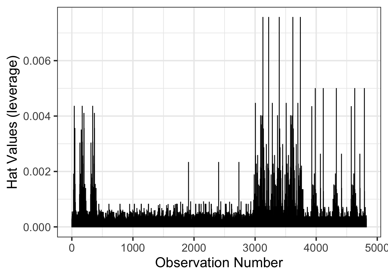

plot(air_lm, which = 1:5)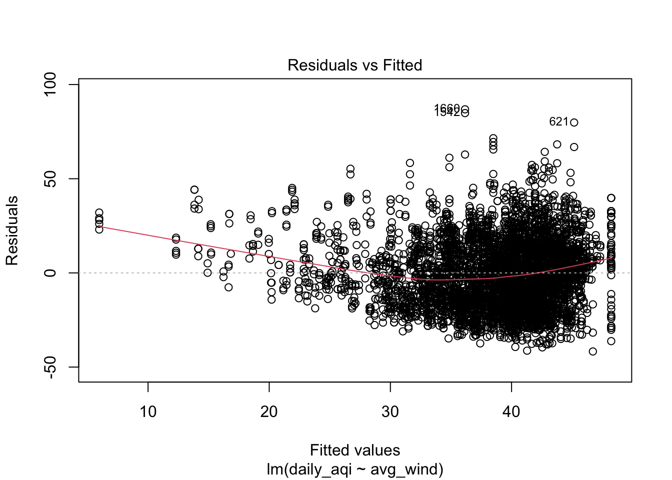

Solutions to overcome data conditions not being met

There are some strategies that can be done when a variety of data conditions for linear regression have not been met. In general, the strategies stem around generalizing the model and adding some complexity.

The following are options that would be possible:

Add interactions or other non-linear terms
Use more complicated model
- weighted least squares for homogeneity of variance concerns
- models that include measurement error
- mixed models for correlated data
Transform the data.

Last updated on Feb 15, 2024