Linear Regression - Activity
In Class Activity - February 1st, 2024
This activity is meant to give you some exploration of topics within class. I’ve created the code for you to run the activity and explore some data.
The goals of this activity are as follows:
- Explore what happens if the X and Y attributes are flipped in a linear regression.
- What happens to the linear regression coefficient estimates (ie., the \(\hat{\beta}\))?
- What happens to the sigma and R-Square statistics?
- Given what you find in #1, how do you decide which attribute should be an outcome (Y) vs a predictor (X)?
library(tidyverse)## ── Attaching core tidyverse packages ──────────────────────── tidyverse 2.0.0 ──
## ✔ dplyr 1.1.4 ✔ readr 2.1.5
## ✔ forcats 1.0.0 ✔ stringr 1.5.1
## ✔ ggplot2 3.4.4 ✔ tibble 3.2.1
## ✔ lubridate 1.9.3 ✔ tidyr 1.3.1
## ✔ purrr 1.0.2
## ── Conflicts ────────────────────────────────────────── tidyverse_conflicts() ──
## ✖ dplyr::filter() masks stats::filter()
## ✖ dplyr::lag() masks stats::lag()
## ℹ Use the conflicted package (<http://conflicted.r-lib.org/>) to force all conflicts to become errorslibrary(palmerpenguins)
library(ggformula)## Loading required package: scales
##
## Attaching package: 'scales'
##
## The following object is masked from 'package:purrr':
##
## discard
##
## The following object is masked from 'package:readr':
##
## col_factor
##
## Loading required package: ggridges
##
## New to ggformula? Try the tutorials:
## learnr::run_tutorial("introduction", package = "ggformula")
## learnr::run_tutorial("refining", package = "ggformula")library(mosaic)## Registered S3 method overwritten by 'mosaic':
## method from
## fortify.SpatialPolygonsDataFrame ggplot2
##
## The 'mosaic' package masks several functions from core packages in order to add
## additional features. The original behavior of these functions should not be affected by this.
##
## Attaching package: 'mosaic'
##
## The following object is masked from 'package:Matrix':
##
## mean
##
## The following object is masked from 'package:scales':
##
## rescale
##
## The following objects are masked from 'package:dplyr':
##
## count, do, tally
##
## The following object is masked from 'package:purrr':
##
## cross
##
## The following object is masked from 'package:ggplot2':
##
## stat
##
## The following objects are masked from 'package:stats':
##
## binom.test, cor, cor.test, cov, fivenum, IQR, median, prop.test,
## quantile, sd, t.test, var
##
## The following objects are masked from 'package:base':
##
## max, mean, min, prod, range, sample, sumtheme_set(theme_bw(base_size = 16))
# If you get errors, use this line of code too.
# penguins <- readr::read_csv("https://raw.githubusercontent.com/allisonhorst/palmerpenguins/main/inst/extdata/penguins.csv")
head(penguins)## # A tibble: 6 × 8
## species island bill_length_mm bill_depth_mm flipper_length_mm body_mass_g
## <fct> <fct> <dbl> <dbl> <int> <int>
## 1 Adelie Torgersen 39.1 18.7 181 3750
## 2 Adelie Torgersen 39.5 17.4 186 3800
## 3 Adelie Torgersen 40.3 18 195 3250
## 4 Adelie Torgersen NA NA NA NA
## 5 Adelie Torgersen 36.7 19.3 193 3450
## 6 Adelie Torgersen 39.3 20.6 190 3650
## # ℹ 2 more variables: sex <fct>, year <int>model_fit <- function(outcome, predictor, data = penguins) {
formula <- as.formula(paste(outcome, predictor, sep = "~"))
model_out <- lm(formula, data = data)
model_coef <- data.frame(matrix(c(coef(model_out)), ncol = 2))
names(model_coef) <- c("Intercept", "Slope")
data.frame(model_coef,
Rsquare = summary(model_out)$r.square,
sigma = summary(model_out)$sigma)
}
visualize_relationship <- function(outcome, predictor, data = penguins,
add_regression_line = TRUE, add_smoother_line = FALSE) {
formula <- as.formula(paste(outcome, predictor, sep = "~"))
if(add_regression_line & !add_smoother_line) {
gf_point(gformula = formula, data = data, size = 4) |>
gf_smooth(method = 'lm', size = 1.5) |> print()
}
if(add_smoother_line & !add_regression_line) {
gf_point(gformula = formula, data = data, size = 4) |>
gf_smooth(method = 'loess', size = 1.5) |> print()
}
if(add_smoother_line & add_regression_line) {
gf_point(gformula = formula, data = data, size = 4) |>
gf_smooth(method = 'lm', size = 1.5) |>
gf_smooth(method = 'loess', size = 1.5, linetype = 2) |> print()
}
}Compute Correlation
The following code chunk can help you compute correlations between attributes. To use the function, you can replace “outcome” with an attribute name from the data above and “predictor” with another attribute above.
- What happens when you flip the outcome / predictor outcomes when computing the correlation? Does the correlation change? Why or why not?
- Given the correlation computed, how is it interpreted?
- Given the correlation computed, what information would this tell us when we try estimate the regression coefficients below?
cor(outcome ~ predictor, data = penguins, use = 'complete.obs') |> round(3)Visualize bivariate distribution
The following code creates a scatter plot showing the bivariate association between the two attributes entered. Example code is shown below as an example. You can replace the “outcome” and “predictor” with the two continuous attributes that you are interested in exploring. These need to be entered in quotations, either single or double are fine. You can also add a regression line or smoother line by specifying those arguments as either TRUE (ie., Yes) or FALSE (ie., No).
- Does the association between the two attributes appear to be linear?
- What happens to the association if you flip the predictor / outcome attributes?
- How would you summarize the association in a few sentences?
visualize_relationship(outcome = 'body_mass_g',
          predictor = 'flipper_length_mm',
          data = penguins,
          add_regression_line = TRUE,
          add_smoother_line = FALSE)
## Warning: Using `size` aesthetic for lines was deprecated in ggplot2 3.4.0.
## ℹ Please use `linewidth` instead.
## This warning is displayed once every 8 hours.
## Call `lifecycle::last_lifecycle_warnings()` to see where this warning was
## generated.## Warning: Removed 2 rows containing non-finite values (`stat_smooth()`).## Warning: Removed 2 rows containing missing values (`geom_point()`).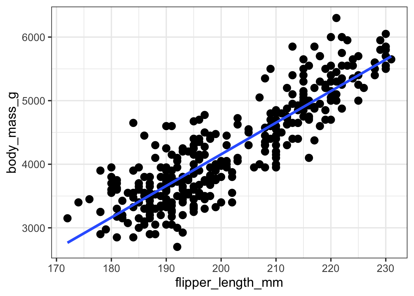
visualize_relationship(outcome = 'flipper_length_mm',
          predictor = 'body_mass_g',
          data = penguins,
          add_regression_line = TRUE,
          add_smoother_line = FALSE)
## Warning: Removed 2 rows containing non-finite values (`stat_smooth()`).## Warning: Removed 2 rows containing missing values (`geom_point()`).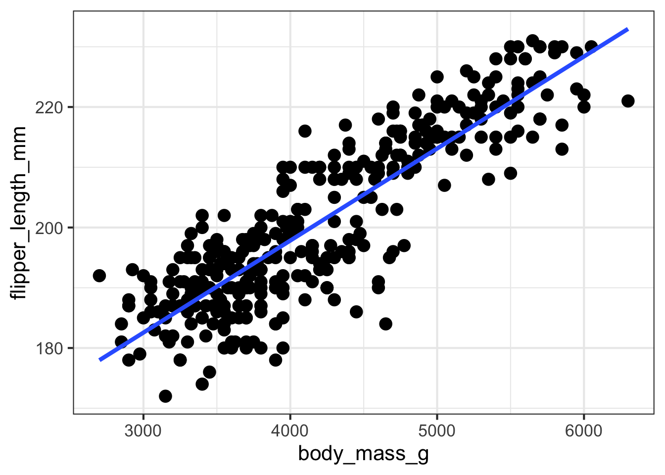
Linear Regression Fitting
Similar to the bivariate scatterplot, the following function was created to fit a linear regression and extract some information about the model. The output should include the Intercept, Slope, R-square, and sigma estimates. You can specify the outcome and predictor by replacing those as you did in the bivariate scatterplot above to reflect the attributes you are interested in exploring.
- How are the 4 estimates interpreted, particularly in the context of the problem?
- What happens to the 4 estimates if you flip the outcome and predictor attributes?
- Which one should truly be the outcome and what should guide this?
model_fit(outcome = 'body_mass_g',
          predictor = 'flipper_length_mm',
          data = penguins)
## Intercept Slope Rsquare sigma
## 1 -5780.831 49.68557 0.7589925 394.2782\[ body\_mass = \beta_{0} + \beta_{1} flipper\_length \]
model_fit(outcome = 'flipper_length_mm',
          predictor = 'body_mass_g',
          data = penguins)
## Intercept Slope Rsquare sigma
## 1 136.7296 0.01527592 0.7589925 6.913393\[ flipper\_length = \beta_{0} + \beta_{1} body\_mass \]