Regression with Categorical Predictors

Regression with Categorical Predictors - class

This set of notes will explore using linear regression for a single predictor attribute that is categorical instead of continuous. To explore this first, let’s explore some data.

# install.packages("Lahman")

# install.packages("Lahman")

library(tidyverse)

## ── Attaching core tidyverse packages ──────────────────────── tidyverse 2.0.0 ──
## ✔ dplyr     1.1.4     ✔ readr     2.1.5
## ✔ forcats   1.0.0     ✔ stringr   1.5.1
## ✔ ggplot2   3.4.4     ✔ tibble    3.2.1
## ✔ lubridate 1.9.3     ✔ tidyr     1.3.1
## ✔ purrr     1.0.2     
## ── Conflicts ────────────────────────────────────────── tidyverse_conflicts() ──
## ✖ dplyr::filter() masks stats::filter()
## ✖ dplyr::lag()    masks stats::lag()
## ℹ Use the conflicted package (<http://conflicted.r-lib.org/>) to force all conflicts to become errors

library(Lahman)
library(ggformula)

## Loading required package: scales
## 
## Attaching package: 'scales'
## 
## The following object is masked from 'package:purrr':
## 
##     discard
## 
## The following object is masked from 'package:readr':
## 
##     col_factor
## 
## Loading required package: ggridges
## 
## New to ggformula?  Try the tutorials: 
## 	learnr::run_tutorial("introduction", package = "ggformula")
## 	learnr::run_tutorial("refining", package = "ggformula")

theme_set(theme_bw(base_size = 18))

career <- Batting |>
  filter(AB > 100) |>
  anti_join(Pitching, by = "playerID") |>
  filter(yearID > 1990) |>
  group_by(playerID, lgID) |>
  summarise(H = sum(H), AB = sum(AB)) |>
  mutate(average = H / AB)

## `summarise()` has grouped output by 'playerID'. You can override using the
## `.groups` argument.

career <- People |>
  tbl_df() |>
  dplyr::select(playerID, nameFirst, nameLast) |>
  unite(name, nameFirst, nameLast, sep = " ") |>
  inner_join(career, by = "playerID") |>
  dplyr::select(-playerID)

## Warning: `tbl_df()` was deprecated in dplyr 1.0.0.
## ℹ Please use `tibble::as_tibble()` instead.
## Call `lifecycle::last_lifecycle_warnings()` to see where this warning was
## generated.

head(career)

## # A tibble: 6 × 5
##   name               lgID      H    AB average
##   <chr>              <fct> <int> <int>   <dbl>
## 1 Jeff Abbott        AL      127   459   0.277
## 2 Kurt Abbott        AL       33   123   0.268
## 3 Kurt Abbott        NL      455  1780   0.256
## 4 Reggie Abercrombie NL       54   255   0.212
## 5 Brent Abernathy    AL      194   767   0.253
## 6 Shawn Abner        AL       81   309   0.262

nrow(career)

## [1] 2938

Question

Suppose we are interested in the batting average of baseball players since 1990, that is, the average is:

\[ average = \frac{number\ of\ hits}{number\ of\ atbats} \]

Let’s first visualize this.

gf_density(~ average, data = career) |>
  gf_labs(x = "Batting Average")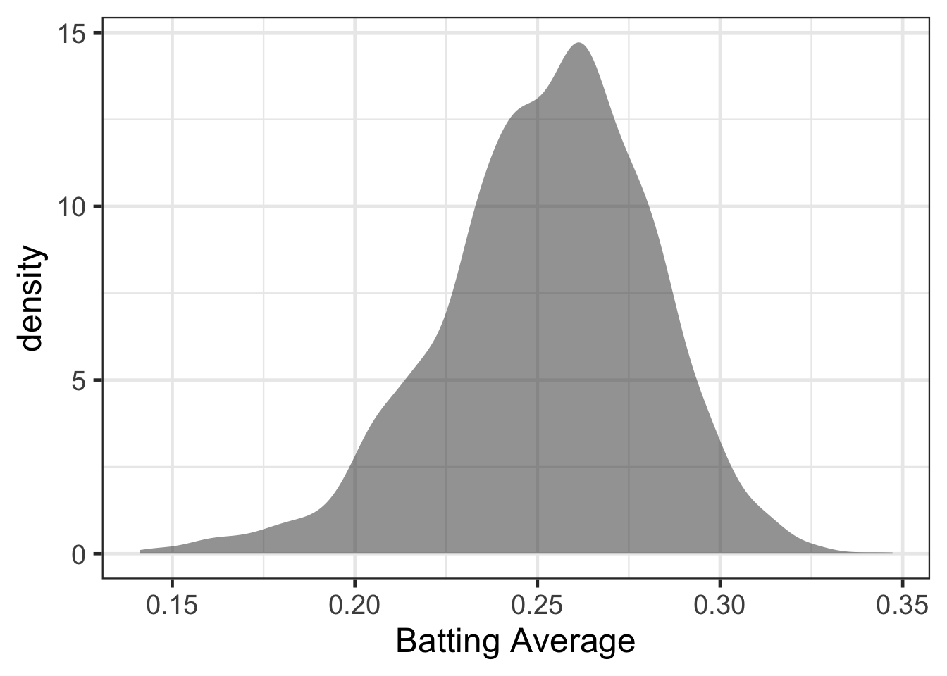

What if we hypothesized that the batting average will differ based on the league that players played in.

gf_violin(lgID ~ average, data = career, fill = 'gray80', draw_quantiles = c('0.1', '0.5', '0.9')) |>
  gf_labs(x = "Batting Average",
          y = "League")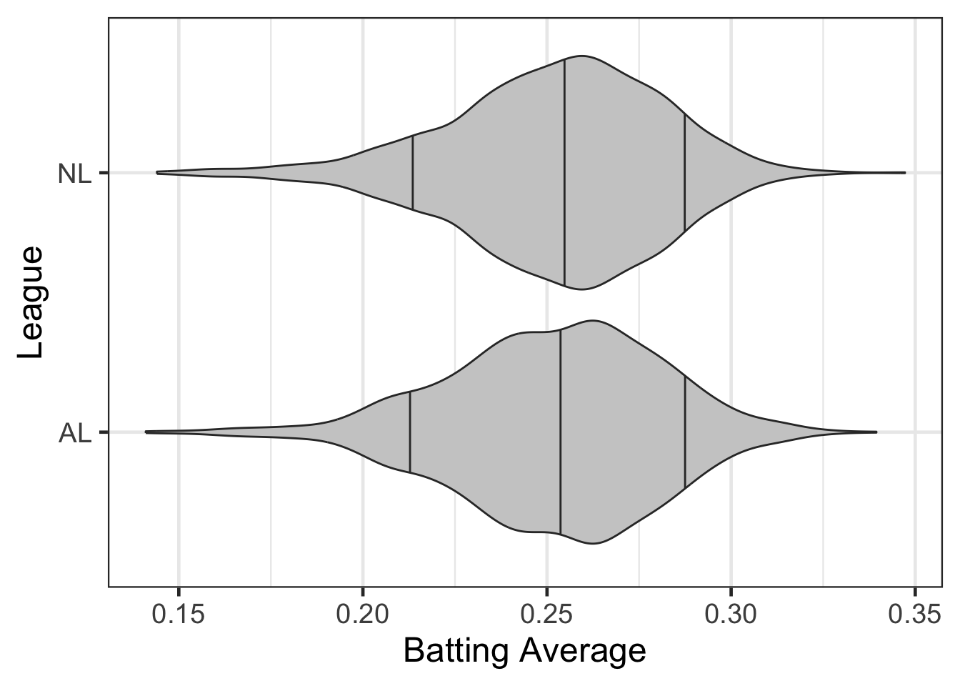

The distributions seem similar, but what if we wanted to go a step further and estimate a model to explore if there are really differences or not. For example, suppose we were interested in:

\[ H_{0}: \mu_{NL} = \mu_{AL} \]

\[ H_{0}: \mu_{NL} - \mu_{AL} = 0 \]

What type of model could we use? What about linear regression?

Linear Regression with Categorical Attributes

Since these notes are happening, you can assume it is possible. But how can a categorical attribute with categories rather than numbers be included in the linear regression model?

The answer is that they can’t. We need a new representation of the categorical attribute, enter dummy or indicator coding.

Dummy/Indicator Coding

Suppose we use the following logic:

If NL, then give a value of 1, else give a value of 0.

Does this give the same information as before?

League ID	Dummy League ID
AL	0
NL	1

What would this look like for the actual data?

career <- career |>
  mutate(league_dummy = ifelse(lgID == 'NL', 1, 0))

head(career, n = 10)

## # A tibble: 10 × 6
##    name               lgID      H    AB average league_dummy
##    <chr>              <fct> <int> <int>   <dbl>        <dbl>
##  1 Jeff Abbott        AL      127   459   0.277            0
##  2 Kurt Abbott        AL       33   123   0.268            0
##  3 Kurt Abbott        NL      455  1780   0.256            1
##  4 Reggie Abercrombie NL       54   255   0.212            1
##  5 Brent Abernathy    AL      194   767   0.253            0
##  6 Shawn Abner        AL       81   309   0.262            0
##  7 Shawn Abner        NL       19   115   0.165            1
##  8 CJ Abrams          NL       70   284   0.246            1
##  9 Bobby Abreu        AL      858  3061   0.280            0
## 10 Bobby Abreu        NL     1602  5373   0.298            1

Now that there is a numeric attribute, these can be added into the linear regression model.

average_lm <- lm(average ~ league_dummy, 
                 data = career)

broom::tidy(average_lm)

## # A tibble: 2 × 5
##   term         estimate std.error statistic p.value
##   <chr>           <dbl>     <dbl>     <dbl>   <dbl>
## 1 (Intercept)  0.252     0.000758   333.      0    
## 2 league_dummy 0.000558  0.00107      0.522   0.602

\[ average = \beta_{0} + \beta_{1} League + \epsilon \]

0.251895 + .00056 *0

## [1] 0.251895

0.251895 + .00056 *1

## [1] 0.252455

How are these terms interpreted now?

df_stats(average ~ league_dummy, data = career, mean, sd, length)

##   response league_dummy      mean         sd length
## 1  average            0 0.2518959 0.02895094   1461
## 2  average            1 0.2524535 0.02896021   1477

average_lm2 <- lm(average ~ lgID, data = career)

broom::tidy(average_lm2) |> mutate_if(is.double, round, 3)

## # A tibble: 2 × 5
##   term        estimate std.error statistic p.value
##   <chr>          <dbl>     <dbl>     <dbl>   <dbl>
## 1 (Intercept)    0.252     0.001   333.      0    
## 2 lgIDNL         0.001     0.001     0.522   0.602

confint(average_lm2)

##                   2.5 %      97.5 %
## (Intercept)  0.25041049 0.253381234
## lgIDNL      -0.00153733 0.002652537

t.test(average ~ lgID, 
       data = career, 
       var.equal = TRUE)

## 
## 	Two Sample t-test
## 
## data:  average by lgID
## t = -0.52189, df = 2936, p-value = 0.6018
## alternative hypothesis: true difference in means between group AL and group NL is not equal to 0
## 95 percent confidence interval:
##  -0.002652537  0.001537330
## sample estimates:
## mean in group AL mean in group NL 
##        0.2518959        0.2524535

Values other than 0/1

First, I want to build off of the first part of the notes on regression with categorical predictors. Before generalizing to more than two groups, let’s first explore what happens when values other than 0/1 are used for the categorical attribute. The following three dummy/indicator attributes will be used:

1 = NL, 0 = AL
1 = NL, 2 = AL
100 = NL, 0 = AL

Make some predictions about what you think will happen in the three separate regressions?

library(tidyverse)
library(Lahman)
library(ggformula)

theme_set(theme_bw(base_size = 18))

career <- Batting |>
  filter(AB > 100) |>
  anti_join(Pitching, by = "playerID") |>
  filter(yearID > 1990) |>
  group_by(playerID, lgID) |>
  summarise(H = sum(H), AB = sum(AB)) |>
  mutate(average = H / AB)

## `summarise()` has grouped output by 'playerID'. You can override using the
## `.groups` argument.

career <- People |>
  tbl_df() |>
  dplyr::select(playerID, nameFirst, nameLast) |>
  unite(name, nameFirst, nameLast, sep = " ") |>
  inner_join(career, by = "playerID") |>
  dplyr::select(-playerID)

## Warning: `tbl_df()` was deprecated in dplyr 1.0.0.
## ℹ Please use `tibble::as_tibble()` instead.
## Call `lifecycle::last_lifecycle_warnings()` to see where this warning was
## generated.

career <- career |>
  mutate(league_dummy = ifelse(lgID == 'NL', 0, 1),
         league_dummy_12 = ifelse(lgID == 'NL', 1, 2),
         league_dummy_100 = ifelse(lgID == 'NL', 100, 0))

head(career, n = 10)

## # A tibble: 10 × 8
##    name  lgID      H    AB average league_dummy league_dummy_12 league_dummy_100
##    <chr> <fct> <int> <int>   <dbl>        <dbl>           <dbl>            <dbl>
##  1 Jeff… AL      127   459   0.277            1               2                0
##  2 Kurt… AL       33   123   0.268            1               2                0
##  3 Kurt… NL      455  1780   0.256            0               1              100
##  4 Regg… NL       54   255   0.212            0               1              100
##  5 Bren… AL      194   767   0.253            1               2                0
##  6 Shaw… AL       81   309   0.262            1               2                0
##  7 Shaw… NL       19   115   0.165            0               1              100
##  8 CJ A… NL       70   284   0.246            0               1              100
##  9 Bobb… AL      858  3061   0.280            1               2                0
## 10 Bobb… NL     1602  5373   0.298            0               1              100

average_lm <- lm(average ~ league_dummy, data = career)

broom::tidy(average_lm)|> mutate_if(is.double, round, 4)

## # A tibble: 2 × 5
##   term         estimate std.error statistic p.value
##   <chr>           <dbl>     <dbl>     <dbl>   <dbl>
## 1 (Intercept)    0.252     0.0008   335.      0    
## 2 league_dummy  -0.0006    0.0011    -0.522   0.602

average_lm_12 <- lm(average ~ league_dummy_12, data = career)

broom::tidy(average_lm_12)|> mutate_if(is.double, round, 4)

## # A tibble: 2 × 5
##   term            estimate std.error statistic p.value
##   <chr>              <dbl>     <dbl>     <dbl>   <dbl>
## 1 (Intercept)       0.253     0.0017   150.      0    
## 2 league_dummy_12  -0.0006    0.0011    -0.522   0.602

average_lm_100 <- lm(average ~ league_dummy_100, data = career)

broom::tidy(average_lm_100)|> mutate_if(is.double, round, 5)

## # A tibble: 2 × 5
##   term             estimate std.error statistic p.value
##   <chr>               <dbl>     <dbl>     <dbl>   <dbl>
## 1 (Intercept)       0.252     0.00076   333.      0    
## 2 league_dummy_100  0.00001   0.00001     0.522   0.602

Before moving to more than 2 groups, any thoughts on how we could run a one-sample t-test using a linear regression? For example, suppose this null hypothesis wanted to be explored.

\[ H_{0}: \mu_{BA} = .2 \]

\[ H_{A}: \mu_{BA} \neq .2 \]

t.test(career$average, mu = .2)

## 
## 	One Sample t-test
## 
## data:  career$average
## t = 97.683, df = 2937, p-value < 2.2e-16
## alternative hypothesis: true mean is not equal to 0.2
## 95 percent confidence interval:
##  0.2511289 0.2532235
## sample estimates:
## mean of x 
## 0.2521762

broom::tidy(
    lm(average ~ 1, data = career)
    )

## # A tibble: 1 × 5
##   term        estimate std.error statistic p.value
##   <chr>          <dbl>     <dbl>     <dbl>   <dbl>
## 1 (Intercept)    0.252  0.000534      472.       0

(0.2521762 - 0.2) / 0.0005342373

## [1] 97.66484

broom::tidy(
    lm(I(average - 0.2) ~ 1, data = career)
    )

## # A tibble: 1 × 5
##   term        estimate std.error statistic p.value
##   <chr>          <dbl>     <dbl>     <dbl>   <dbl>
## 1 (Intercept)   0.0522  0.000534      97.7       0

\[ H_{0}: \beta_{0} = 0 \]

Generalize to more than 2 groups

The ability to use regression with categorical attributes of more than 2 groups is possible and an extension of the 2 groups model shown above. First, let’s think about how we could represent three categories as numeric attributes. Suppose we had the following 4 categories of baseball players.

Position	option 1	Option 2	infield	outfield	catcher
Outfield	0	1	0	1	0
Infield	1	2	1	0	0
Catcher	2	0	0	0	1
Designated Hitter	3	3	0	0	0

remotes::install_github("bdilday/GeomMLBStadiums")

## Skipping install of 'GeomMLBStadiums' from a github remote, the SHA1 (90b4356e) has not changed since last install.
##   Use `force = TRUE` to force installation

library(GeomMLBStadiums)

ggplot() + 
   geom_mlb_stadium(stadium_ids = "yankees", 
                   stadium_segments = "all") + 
  facet_wrap(~team) + 
  coord_fixed() + 
  theme_void()

library(tidyverse)
library(Lahman)
library(ggformula)

theme_set(theme_bw(base_size = 18))

career <- Batting |>
  filter(AB > 100) |>
  anti_join(Pitching, by = "playerID") |>
  filter(yearID > 1990) |>
  group_by(playerID, lgID) |>
  summarise(H = sum(H), AB = sum(AB)) |>
  mutate(average = H / AB)

## `summarise()` has grouped output by 'playerID'. You can override using the
## `.groups` argument.

career <- Appearances |>
  filter(yearID > 1990) |>
  select(-GS, -G_ph, -G_pr, -G_batting, -G_defense, -G_p, -G_lf, -G_cf, -G_rf) |>
  rowwise() |>
  mutate(g_inf = sum(c_across(G_1b:G_ss))) |>
  select(-G_1b, -G_2b, -G_3b, -G_ss) |>
  group_by(playerID, lgID) |>
  summarise(catcher = sum(G_c),
            outfield = sum(G_of),
            dh = sum(G_dh),
            infield = sum(g_inf),
            total_games = sum(G_all)) |>
  pivot_longer(catcher:infield,
               names_to = "position") |>
  filter(value > 0) |>
  group_by(playerID, lgID) |>
  slice_max(value) |>
  select(playerID, lgID, position) |>
  inner_join(career)

## `summarise()` has grouped output by 'playerID'. You can override using the
## `.groups` argument.
## Joining with `by = join_by(playerID, lgID)`

career <- People |>
  tbl_df() |>
  dplyr::select(playerID, nameFirst, nameLast) |>
  unite(name, nameFirst, nameLast, sep = " ") |>
  inner_join(career, by = "playerID")

## Warning: `tbl_df()` was deprecated in dplyr 1.0.0.
## ℹ Please use `tibble::as_tibble()` instead.
## Call `lifecycle::last_lifecycle_warnings()` to see where this warning was
## generated.

career <- career |>
  mutate(league_dummy = ifelse(lgID == 'NL', 1, 0))

count(career, position)

## # A tibble: 4 × 2
##   position     n
##   <chr>    <int>
## 1 catcher    415
## 2 dh          83
## 3 infield   1279
## 4 outfield  1165

gf_violin(position ~ average, data = career, fill = 'gray85', draw_quantiles = c(0.1, 0.5, 0.9)) |>
  gf_labs(x = "Batting Average",
          y = "")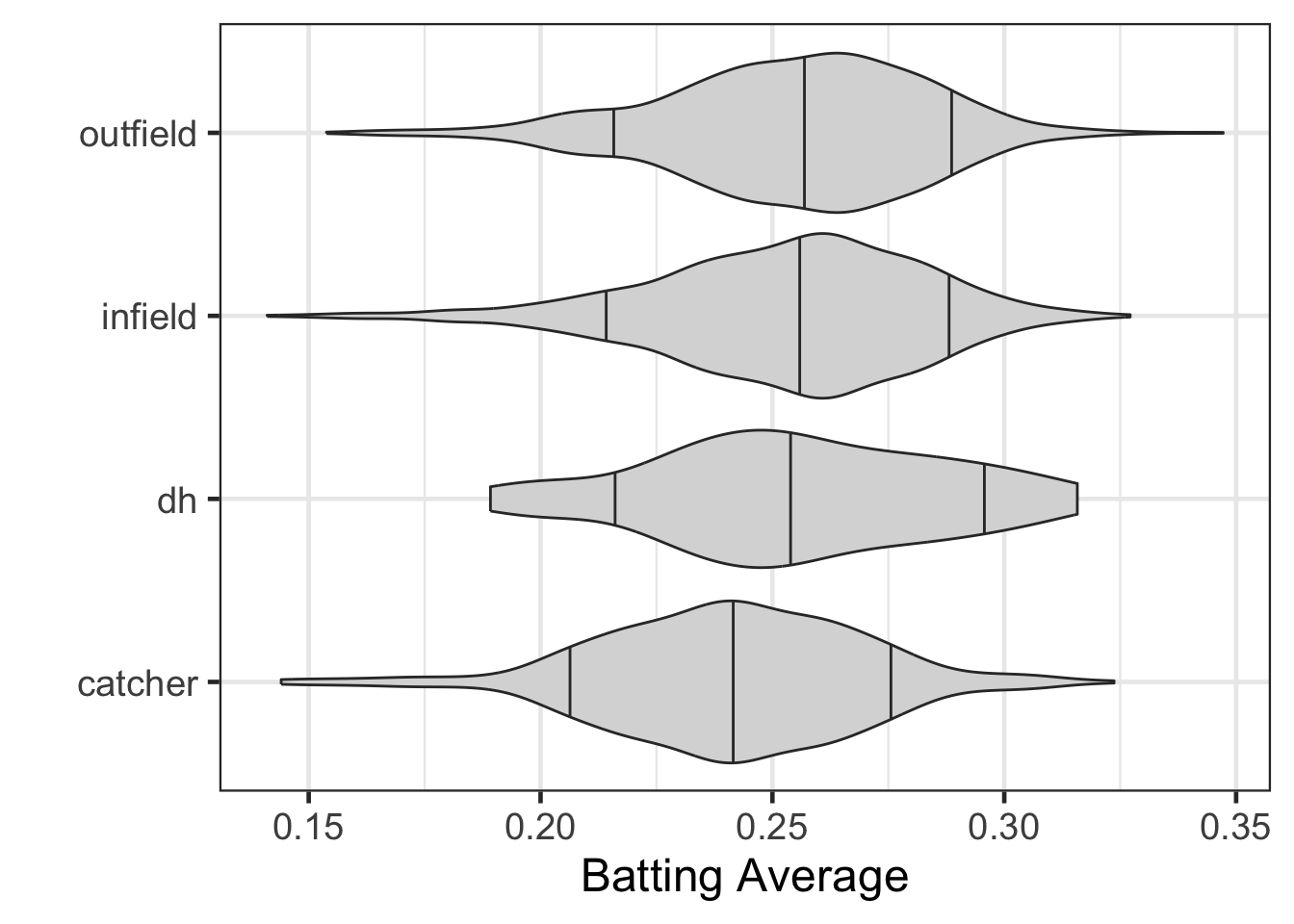

career <- career |> 
mutate(position_num = ifelse(position == 'catcher', 0, ifelse(position == 'infield', 1, ifelse(position == 'outfield', 2, 3))))

count(career, position, position_num)

## # A tibble: 4 × 3
##   position position_num     n
##   <chr>           <dbl> <int>
## 1 catcher             0   415
## 2 dh                  3    83
## 3 infield             1  1279
## 4 outfield            2  1165

broom::tidy(
    lm(average ~ position_num, data = career)
    )

## # A tibble: 2 × 5
##   term         estimate std.error statistic  p.value
##   <chr>           <dbl>     <dbl>     <dbl>    <dbl>
## 1 (Intercept)   0.246    0.00107     229.   0       
## 2 position_num  0.00505  0.000712      7.10 1.60e-12

gf_jitter(average ~ position_num, data = career, size = 4) |> 
gf_smooth(method = 'lm')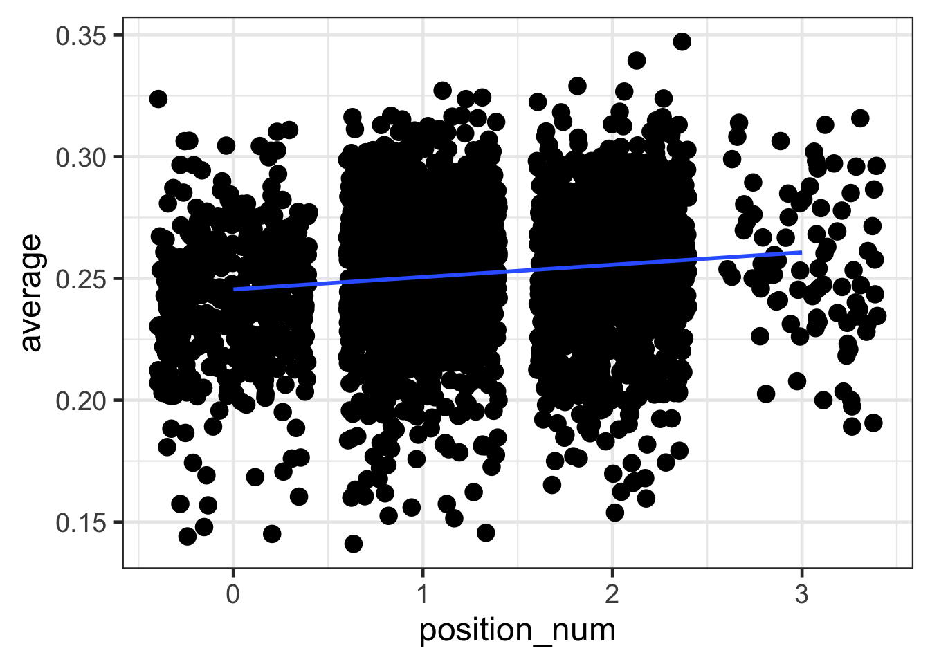

career <- career |>
  mutate(outfield = ifelse(position == 'outfield', 1, 0),
         infield = ifelse(position == 'infield', 1, 0),
         catcher = ifelse(position == 'catcher', 1, 0))

head(career)

## # A tibble: 6 × 12
##   playerID  name    lgID  position     H    AB average league_dummy position_num
##   <chr>     <chr>   <fct> <chr>    <int> <int>   <dbl>        <dbl>        <dbl>
## 1 abbotje01 Jeff A… AL    outfield   127   459   0.277            0            2
## 2 abbotku01 Kurt A… AL    infield     33   123   0.268            0            1
## 3 abbotku01 Kurt A… NL    infield    455  1780   0.256            1            1
## 4 abercre01 Reggie… NL    outfield    54   255   0.212            1            2
## 5 abernbr01 Brent … AL    infield    194   767   0.253            0            1
## 6 abnersh01 Shawn … AL    outfield    81   309   0.262            0            2
## # ℹ 3 more variables: outfield <dbl>, infield <dbl>, catcher <dbl>

position_lm <- lm(average ~ 1 + outfield + infield + catcher, data = career)

broom::tidy(position_lm) |> mutate_if(is.double, round, 4)

## # A tibble: 4 × 5
##   term        estimate std.error statistic p.value
##   <chr>          <dbl>     <dbl>     <dbl>   <dbl>
## 1 (Intercept)   0.255     0.0031    81.3     0    
## 2 outfield     -0.0006    0.0033    -0.188   0.851
## 3 infield      -0.0022    0.0032    -0.672   0.501
## 4 catcher      -0.0144    0.0034    -4.19    0

df_stats(average ~ position, data = career, mean)

##   response position      mean
## 1  average  catcher 0.2409461
## 2  average       dh 0.2553577
## 3  average  infield 0.2531783
## 4  average outfield 0.2547475

broom::tidy(
    lm(average ~ position, data = career)
    )

## # A tibble: 4 × 5
##   term             estimate std.error statistic  p.value
##   <chr>               <dbl>     <dbl>     <dbl>    <dbl>
## 1 (Intercept)        0.241    0.00140    172.   0       
## 2 positiondh         0.0144   0.00344      4.19 2.88e- 5
## 3 positioninfield    0.0122   0.00162      7.57 5.03e-14
## 4 positionoutfield   0.0138   0.00164      8.44 4.97e-17

Last updated on Mar 26, 2024