Bootstrapping Steps

The following are the steps when performing a bootstrap.

1. Treat the sample data as the population.
2. Resample, with replacement, from the sample data, ensuring the new sample is the same size as the original.
3. Estimate the model using the resampled data from step 2.
4. Repeat steps 2 and 3 many many times (eg, 10,000 or more).
5. Visualize distribution of effect of interest

Resampling with replacement

What is meant by sampling with replacement? Let’s do an example.

library(tidyverse)

## ── Attaching core tidyverse packages ──────────────────────── tidyverse 2.0.0 ──
## ✔ dplyr     1.1.4     ✔ readr     2.1.5
## ✔ forcats   1.0.0     ✔ stringr   1.5.1
## ✔ ggplot2   3.4.4     ✔ tibble    3.2.1
## ✔ lubridate 1.9.3     ✔ tidyr     1.3.1
## ✔ purrr     1.0.2     
## ── Conflicts ────────────────────────────────────────── tidyverse_conflicts() ──
## ✖ dplyr::filter() masks stats::filter()
## ✖ dplyr::lag()    masks stats::lag()
## ℹ Use the conflicted package (<http://conflicted.r-lib.org/>) to force all conflicts to become errors

fruit <- data.frame(name = c('watermelon', 'apple', 'orange', 
                             'kumquat', 'grapes', 'canteloupe', 
                             'kiwi', 'banana')) |>
    mutate(obs_num = 1:n())

fruit

##         name obs_num
## 1 watermelon       1
## 2      apple       2
## 3     orange       3
## 4    kumquat       4
## 5     grapes       5
## 6 canteloupe       6
## 7       kiwi       7
## 8     banana       8

slice_sample(fruit, n = nrow(fruit), replace = FALSE)

##         name obs_num
## 1      apple       2
## 2     grapes       5
## 3     banana       8
## 4 canteloupe       6
## 5    kumquat       4
## 6     orange       3
## 7       kiwi       7
## 8 watermelon       1

slice_sample(fruit, n = nrow(fruit), replace = TRUE)

##         name obs_num
## 1     banana       8
## 2     grapes       5
## 3    kumquat       4
## 4      apple       2
## 5       kiwi       7
## 6      apple       2
## 7 canteloupe       6
## 8     orange       3

8 ^ 8

## [1] 16777216

4000 ^ 4000

## [1] Inf

More practical example

Let’s load some data to do a more practical example. The following data come from a TIMSS on science achievement. The data provided is a subset of the available data and is not intended to be representative. Below is a short description of the data. Please don’t hesitate to send any data related questions, happy to provide additional help on interpreting the data appropriately.

• IDSTUD: A unique student ID
• ITBIRTHM: The birth month of the student
• ITBIRTHY: The birth year of the student
• ITSEX: The birth sex of the student
• ASDAGE: The age of the student (at time of test)
• ASSSCI01: Overall science scale score
• ASSEAR01: Earth science scale score
• ASSLIF01: Life science scale score
• ASSPHY01: Physics scale score
• ASSKNO01: Science knowing scale score
• ASSAPP01: Science applying scale score
• ASSREA01: Science reasoning scale score

library(tidyverse)

timss <- readr::read_csv('https://raw.githubusercontent.com/lebebr01/psqf_6243/main/data/timss_grade4_science.csv') |> 
   filter(ASDAGE < 15)

## Rows: 10029 Columns: 12
## ── Column specification ────────────────────────────────────────────────────────
## Delimiter: ","
## dbl (12): IDSTUD, ITBIRTHM, ITBIRTHY, ITSEX, ASDAGE, ASSSCI01, ASSEAR01, ASS...
## 
## ℹ Use `spec()` to retrieve the full column specification for this data.
## ℹ Specify the column types or set `show_col_types = FALSE` to quiet this message.

head(timss)

## # A tibble: 6 × 12
##   IDSTUD ITBIRTHM ITBIRTHY ITSEX ASDAGE ASSSCI01 ASSEAR01 ASSLIF01 ASSPHY01
##    <dbl>    <dbl>    <dbl> <dbl>  <dbl>    <dbl>    <dbl>    <dbl>    <dbl>
## 1  10101        6     2005     2   9.92     505.     445.     408.     458.
## 2  10102       10     2005     2   9.58     401.     291.     323.     297.
## 3  10103        1     2005     1  10.3      542.     440.     529.     529.
## 4  10104        6     2005     2   9.92     544.     534.     552.     557.
## 5  10105        6     2005     2   9.92     588.     555.     500.     559.
## 6  10106       12     2005     1   9.42     583.     556.     585.     562.
## # ℹ 3 more variables: ASSKNO01 <dbl>, ASSAPP01 <dbl>, ASSREA01 <dbl>

Two Guiding Questions

1. Is the age of a student related to their overall science scale score?
2. Is the life science scale score related to the overall science scale score?

Bivariate exploration

It is important to explore relationships bivariately before going to the model phase. To do this, fill in the outcome of interest in place of “%%” below and fill in the appropriate predictor in place of “^^”. You may also want to fill in an appropriate axis labels in place of “@@” below.

• Summarize the bivariate association

library(ggformula)

## Loading required package: scales

## 
## Attaching package: 'scales'

## The following object is masked from 'package:purrr':
## 
##     discard

## The following object is masked from 'package:readr':
## 
##     col_factor

## Loading required package: ggridges

## 
## New to ggformula?  Try the tutorials: 
## 	learnr::run_tutorial("introduction", package = "ggformula")
## 	learnr::run_tutorial("refining", package = "ggformula")

theme_set(theme_bw(base_size = 18))

gf_point(ASSSCI01 ~ ASDAGE, data = timss, size = 4, alpha = .15) |> 
  gf_smooth(method = 'lm', size = 1.5) |>
  gf_smooth(method = 'loess', size = 1.5, color = 'green') |>
  gf_labs(x = "Age",
          y = "Science Score")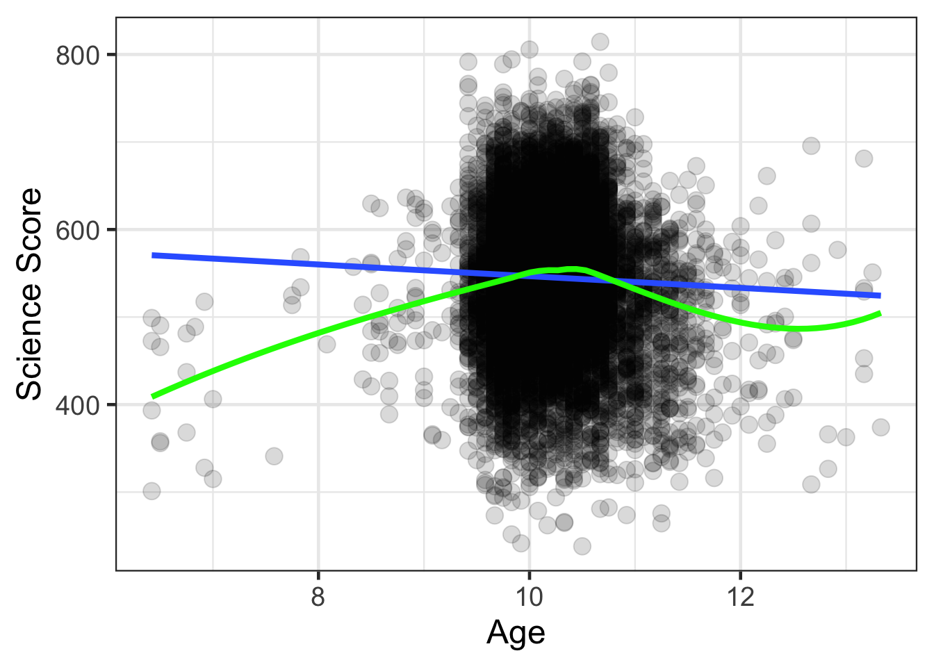

mosaic::cor(ASSSCI01 ~ ASDAGE, data = timss) |> round(5)

## Registered S3 method overwritten by 'mosaic':
##   method                           from   
##   fortify.SpatialPolygonsDataFrame ggplot2

## [1] -0.03999

mosaic::cor(ASSSCI01 ~ ASDAGE, data = filter(timss, ASDAGE >= 8 & ASDAGE <= 12)) |> round(5)

## [1] -0.04989

filter(timss, ASDAGE >= 8 & ASDAGE <= 12) |> nrow()

## [1] 9962

nrow(timss)

## [1] 10027

Estimate Parameters

To do this, fill in the outcome of interest in place of “%%” below and fill in the appropriate predictor in place of “^^”.

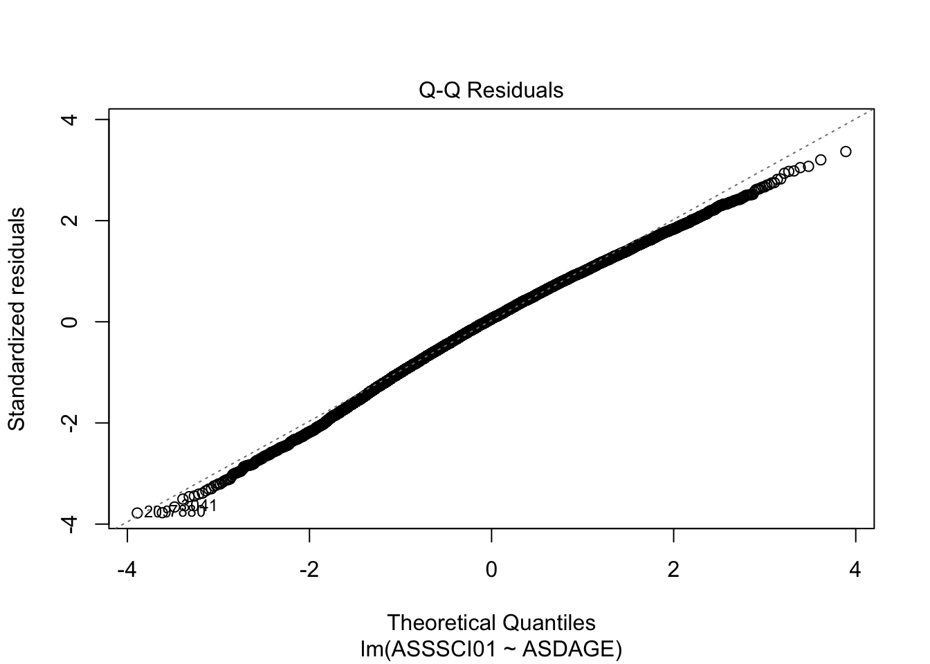
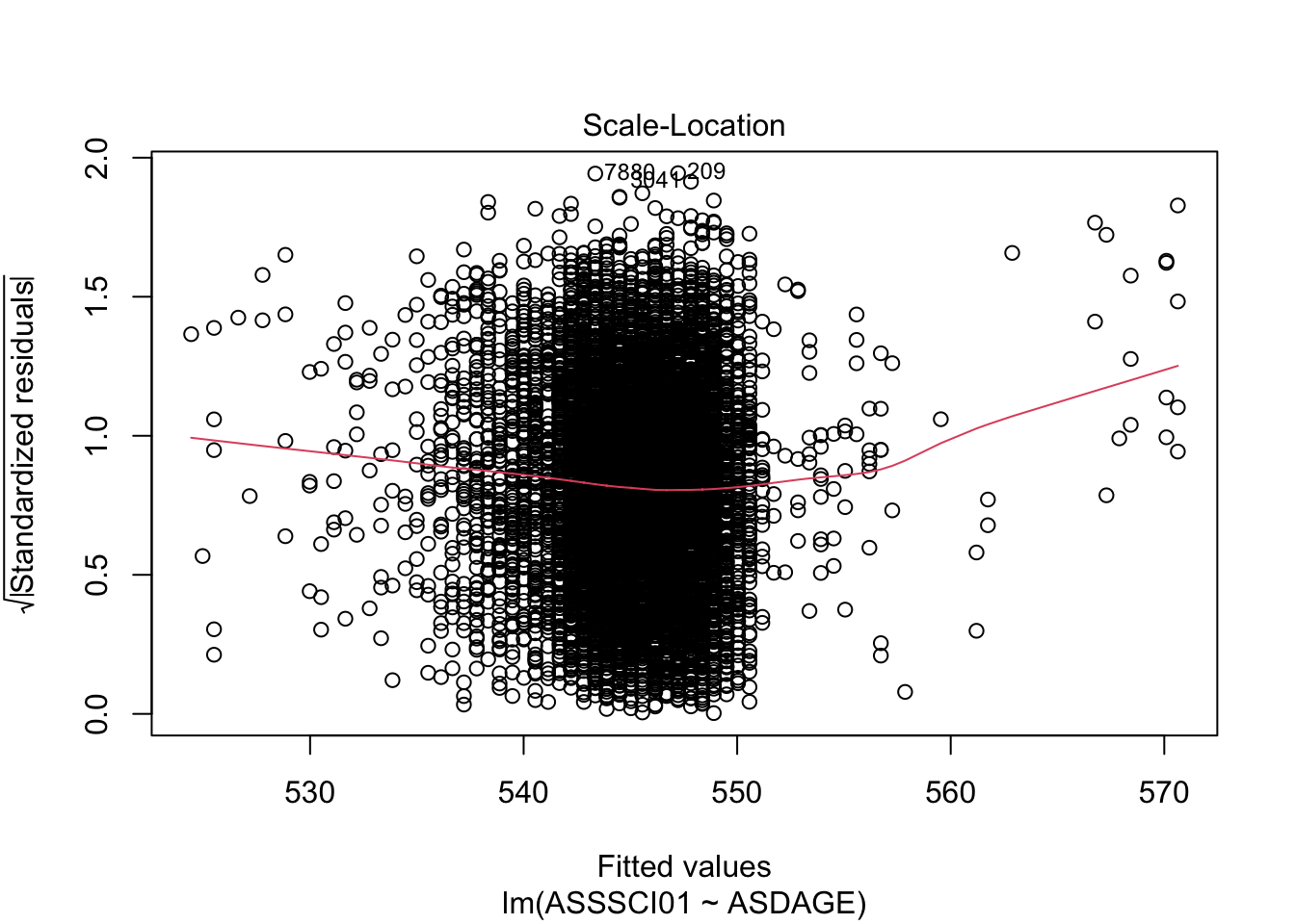
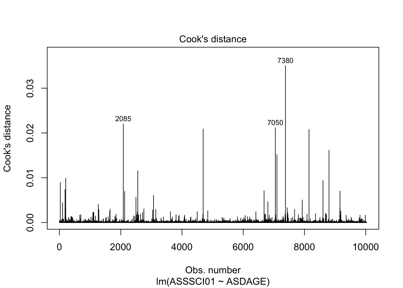
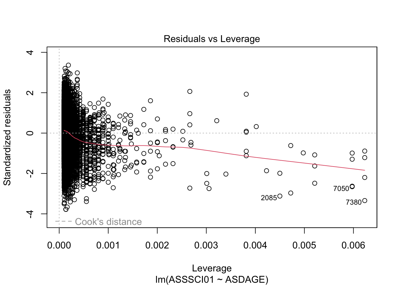
• Interpret the following parameter estimates in the context of the current problem. (ie., what do these parameter estimates mean?)

timss_model <- lm(ASSSCI01 ~ ASDAGE, data = timss)

summary(timss_model)

## 
## Call:
## lm(formula = ASSSCI01 ~ ASDAGE, data = timss)
## 
## Residuals:
##      Min       1Q   Median       3Q      Max 
## -305.769  -51.969    4.919   56.707  272.217 
## 
## Coefficients:
##             Estimate Std. Error t value Pr(>|t|)    
## (Intercept)  613.563     17.064  35.956  < 2e-16 ***
## ASDAGE        -6.687      1.669  -4.007 6.18e-05 ***
## ---
## Signif. codes:  0 '***' 0.001 '**' 0.01 '*' 0.05 '.' 0.1 ' ' 1
## 
## Residual standard error: 80.89 on 10025 degrees of freedom
## Multiple R-squared:  0.001599,	Adjusted R-squared:  0.0015 
## F-statistic: 16.06 on 1 and 10025 DF,  p-value: 6.183e-05

confint(timss_model)

##                  2.5 %     97.5 %
## (Intercept) 580.114047 647.012616
## ASDAGE       -9.957345  -3.415915

plot(timss_model, which = 1:5)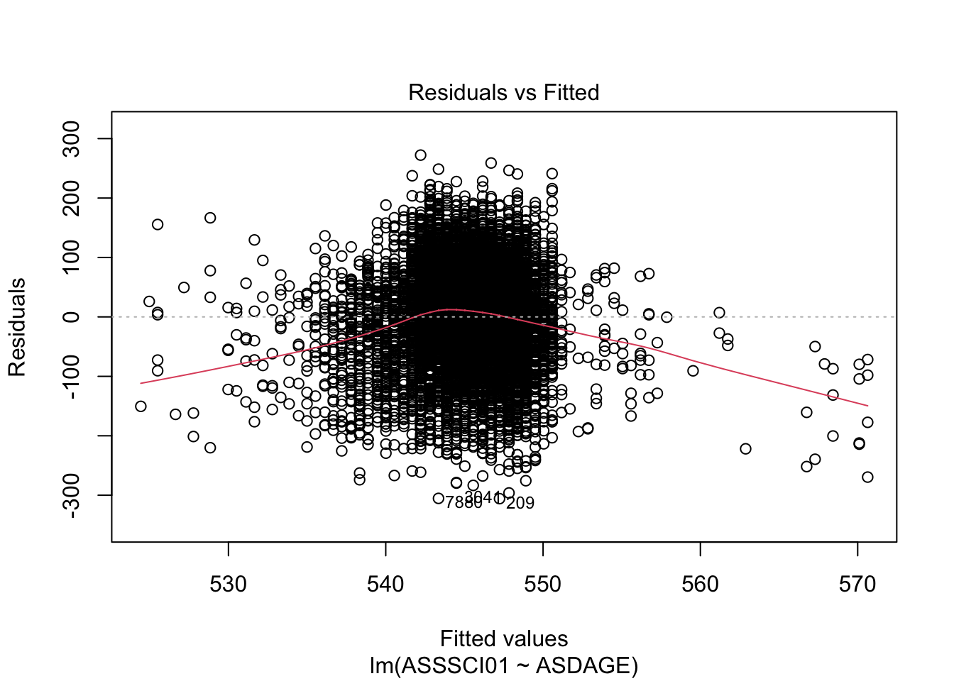

Resample these data

For the astronauts data, to resample, a similar idea can be made. Essentially, we are treating these data as a random sample of some population of space missions. We again, would resample, with replacement, which means that multiple missions would likely show up in the resampling procedure.

slice_sample(timss, n = nrow(timss), replace = TRUE) |> 
  count(IDSTUD) |> 
  arrange(-n)

## # A tibble: 6,332 × 2
##     IDSTUD     n
##      <dbl> <int>
##  1  490109     6
##  2  600202     6
##  3  820316     6
##  4 1010227     6
##  5 1420102     6
##  6 1770214     6
##  7   20410     5
##  8   40417     5
##  9  130204     5
## 10  170205     5
## # ℹ 6,322 more rows

resamp_lm <- slice_sample(timss, n = nrow(timss), replace = TRUE) %>%
  lm(ASSSCI01 ~ ASDAGE, data = .)

summary(resamp_lm)

## 
## Call:
## lm(formula = ASSSCI01 ~ ASDAGE, data = .)
## 
## Residuals:
##      Min       1Q   Median       3Q      Max 
## -305.374  -49.817    4.064   55.371  272.573 
## 
## Coefficients:
##             Estimate Std. Error t value Pr(>|t|)    
## (Intercept)  612.640     17.499  35.010  < 2e-16 ***
## ASDAGE        -6.633      1.712  -3.874 0.000108 ***
## ---
## Signif. codes:  0 '***' 0.001 '**' 0.01 '*' 0.05 '.' 0.1 ' ' 1
## 
## Residual standard error: 80.26 on 10025 degrees of freedom
## Multiple R-squared:  0.001495,	Adjusted R-squared:  0.001395 
## F-statistic: 15.01 on 1 and 10025 DF,  p-value: 0.0001077

confint(resamp_lm)

##                  2.5 %     97.5 %
## (Intercept) 578.338710 646.941301
## ASDAGE       -9.989728  -3.277094

set.seed(2022)

resample_timss <- function(data, model_equation) {
  timss_resample <- slice_sample(data, n = nrow(data), replace = TRUE)
    
  lm(model_equation, data = timss_resample) |>
    coef()
}

resample_timss(data = timss, model_equation = ASSSCI01 ~ ASDAGE)

## (Intercept)      ASDAGE 
##  593.768824   -4.636762

Make sure future.apply is installed

The following code chunk makes sure the future.apply function is installed for parallel processing in R. If you get an error, you can uncomment (delete the # symbol) in the first line of code to (hopefully) install the package yourself.

# install.packages("future.apply")
library(future.apply)

## Loading required package: future

plan(multisession)

Replicate

The following code replicates the analysis many times. Pick an initial value for N and fill in the model equation to match your code above. I will ask you to change this N value later.

timss_coef <- future.apply::future_replicate(10000, resample_timss(data = timss, 
                        model_equation = ASSSCI01 ~ ASDAGE), simplify = FALSE) |>
                        dplyr::bind_rows() |> 
                        tidyr::pivot_longer(cols = everything())

head(timss_coef)

## # A tibble: 6 × 2
##   name         value
##   <chr>        <dbl>
## 1 (Intercept) 610.  
## 2 ASDAGE       -6.56
## 3 (Intercept) 603.  
## 4 ASDAGE       -5.67
## 5 (Intercept) 620.  
## 6 ASDAGE       -7.25

Visualize results

The following code visualizes the results of the analysis above. Explore the following questions.

1. What does this distribution show/represent?
2. What are key features of this distribution?
3. How do these values compare to the original linear regression results?
   • Are there comparable statistics here compared to those?

gf_density(~ value, data = timss_coef) |>
  gf_facet_wrap(~ name, scales = 'free') |>
  gf_labs(x = "Regression Estimates")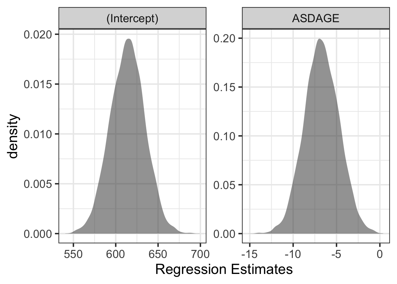

df_stats(value ~ name, data = timss_coef, mean, median, sd, IQR, length)

##   response        name       mean     median        sd       IQR length
## 1    value (Intercept) 613.863905 614.021876 20.493175 27.714280  10000
## 2    value      ASDAGE  -6.714967  -6.740487  2.005943  2.728819  10000

df_stats(value ~ name, data = timss_coef, quantile(c(0.025, 0.975)))

##   response        name      2.5%      97.5%
## 1    value (Intercept) 574.15367 653.425218
## 2    value      ASDAGE -10.57731  -2.829617

confint(timss_model)

##                  2.5 %     97.5 %
## (Intercept) 580.114047 647.012616
## ASDAGE       -9.957345  -3.415915

summary(timss_model)

## 
## Call:
## lm(formula = ASSSCI01 ~ ASDAGE, data = timss)
## 
## Residuals:
##      Min       1Q   Median       3Q      Max 
## -305.769  -51.969    4.919   56.707  272.217 
## 
## Coefficients:
##             Estimate Std. Error t value Pr(>|t|)    
## (Intercept)  613.563     17.064  35.956  < 2e-16 ***
## ASDAGE        -6.687      1.669  -4.007 6.18e-05 ***
## ---
## Signif. codes:  0 '***' 0.001 '**' 0.01 '*' 0.05 '.' 0.1 ' ' 1
## 
## Residual standard error: 80.89 on 10025 degrees of freedom
## Multiple R-squared:  0.001599,	Adjusted R-squared:  0.0015 
## F-statistic: 16.06 on 1 and 10025 DF,  p-value: 6.183e-05

(-6.687 - 0) / 2.0075

## [1] -3.331009

pt(-3.331, df = 10025, lower.tail = TRUE) * 2

## [1] 0.0008684728

Change the N value

Now, change the N value for the replicate step (you can either add a new cell to copy/paste the code or just change it in the code above).

• What happens to the resulting figure when the N increases?
• What value for N seems to be reasonable? Why?